CS180-Proj5-Diffusion
CS180-Proj5-Diffusion
Part A: Using a diffusion model
Theory of diffusion
Variational Auto Encoder (VAE)
For many modalities, we can think of the data we observe as represented or generated by an associated unseen latent variable, which we can denote by random variable \(z\). Mathematically, we can denote \(p(x)\) as the probability of the model generates the real image \(x\). Since the decoder generates image from \(z\), so \(p(x)\) is the marginal probability of joint distribution \(p(x, z)\), i.e. \(p(x)=\int p(\tilde{x}=x|z)p(z)dz\). Obviously it is too hard to integrate all possible \(z\), so another way is to use the equation \(p(x) = \frac{p(x,z)}{p(z|x)}\) to calculate it. Still we cannot get the expression of \(p(z|x)\), so we use a deep neural network to imitate it. That is the encoder, we denote it as \(q_{\phi}(z|x)\), where \(\phi\) is the parameters of encoder.
To measure how close these two distributions are, we use kl divergence:
\[ D_{KL}(q_{\phi}(z|x)||p(z|x)) \]
Unfortunately, we cannot access the real distribution \(p(z|x)\), but we have
\[ \log p(\boldsymbol{x}) = \mathbb{E}_{q_{\boldsymbol{\phi}}(\boldsymbol{z}\mid\boldsymbol{x})}\left[\log\frac{p(\boldsymbol{x}, \boldsymbol{z})}{q_{\boldsymbol{\phi}}(\boldsymbol{z}\mid\boldsymbol{x})}\right] + \mathcal{D}_{\text{KL}}(q_{\boldsymbol{\phi}}(\boldsymbol{z}\mid\boldsymbol{x}) \mid\mid p(\boldsymbol{z}\mid\boldsymbol{x})) \]
where \(\mathbb{E}_{q_{\boldsymbol{\phi}}(\boldsymbol{z}\mid\boldsymbol{x})}\left[\log\frac{p(\boldsymbol{x}, \boldsymbol{z})}{q_{\boldsymbol{\phi}}(\boldsymbol{z}\mid\boldsymbol{x})}\right]\) is known as \(ELBO\) (Evidence Lower Bound). Notice that \(p(x)\) is actually related to the decoder's params \(\theta\), so if we fix the \(\theta\), we have:
\[ \log p(\boldsymbol{x}) = Constant = \boldsymbol{ELBO}(\phi)+KL \]
So to minimize KL, we maximize ELBO.
Variational Diffusion Models
\[ p(\boldsymbol{x}, \boldsymbol{z}_{1:T}) = p(\boldsymbol{z}_T)p_{\boldsymbol{\theta}}(\boldsymbol{x}\mid\boldsymbol{z}_1)\prod_{t=2}^{T}p_{\boldsymbol{\theta}}(\boldsymbol{z}_{t-1}\mid\boldsymbol{z}_{t}) \]
and its posterior is:
\[ q_{\boldsymbol{\phi}}(\boldsymbol{z}_{1:T}\mid\boldsymbol{x}) = q_{\boldsymbol{\phi}}(\boldsymbol{z}_1\mid\boldsymbol{x})\prod_{t=2}^{T}q_{\boldsymbol{\phi}}(\boldsymbol{z}_{t}\mid\boldsymbol{z}_{t-1}) \]
There are 3 key restrictions:
- The latent dimension is exactly equal to the data dimension
- The structure of the latent encoder at each timestep is not learned; it is pre-defined as a linear Gaussian model. In other words, it is a Gaussian distribution centered around the output of the previous timestep
- The Gaussian parameters of the latent encoders vary over time in such a way that the distribution of the latent at final timestep \(T\) is a standard Gaussian
For example, we have a real image which is \(x\), we assume it will finally become a pure gaussian distribution (noise) at \(z_T\) with same size by adding gaussian noise:
This means every \(q_{\phi}(x_t|x_{t-1})\) is a Gaussian, we define it as:
\[ q_{\phi}(x_t|x_{t-1}) = \mathcal{N}(x_t | \sqrt{\alpha_t} x_{t-1}, (1-\alpha_t)\bold{I}) \]
where \(\alpha_t\) is a hyperparameter.
Deliverables (Part A)
Seeds: 42
Part 0: Setup
My prompts:
- a photo of the Great Wall
- a photo of beautiful woman
- a photo of a car
- a photo of a cat
- an oil painting of people around a campfire
- an oil painting of an old lady
- a portrait of Steve Jobs
- a football
- a movie star
- a rainbow flag
- a soft bed
Selected prompts:
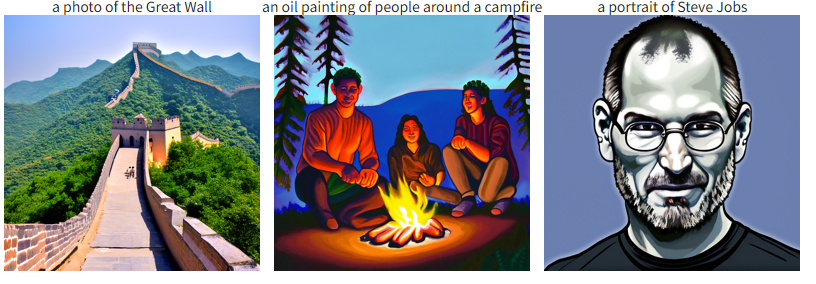
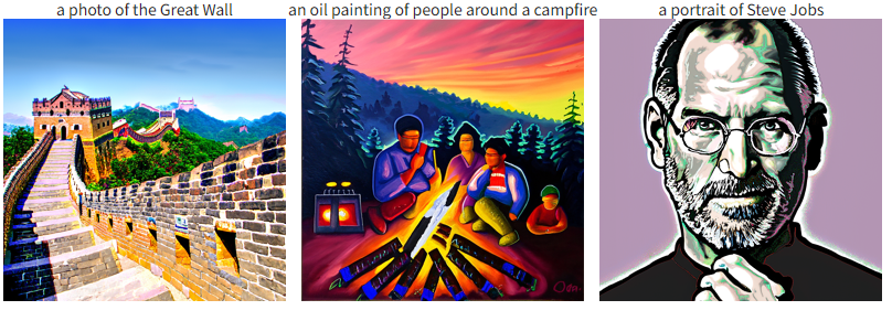
- a photo of the Great Wall
- an oil painting of people around a campfire
- a portrait of Steve Jobs
Results:
num_inference steps = 20
num_inference steps = 200
Part 1: Sampling Loops
Part 1.1: Implementing the Forward Process
- Implement
noisy_im = forward(im, t)function:
1 | |
- Results:
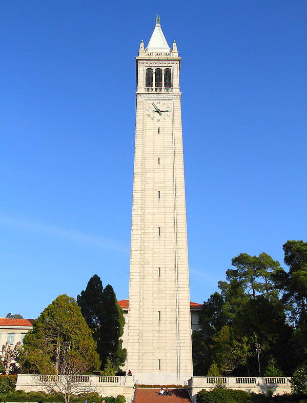
- Original image:
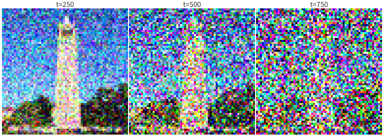
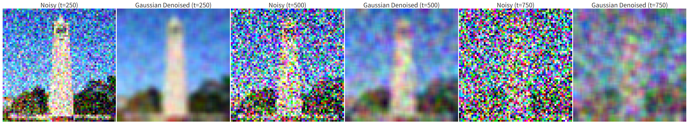
- Noisy image at t=250, 500 and 750:
- Original image:
Part 1.2: Classical Denoising:
- Results:
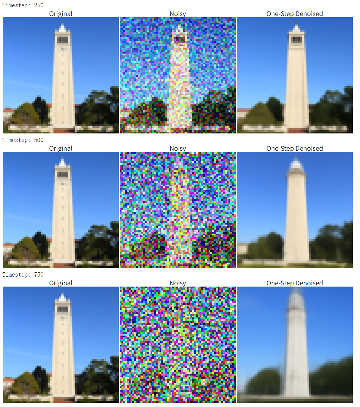
Part 1.3: One-Step Denoising
Using the prompt 'a high quality photo' and a pretrained model to denoise the noisy image at timestep t=250, 500, and 750.
- Results:
Part 1.4: Iterative Denoising
- Results with
i_start = 10andstride = 30: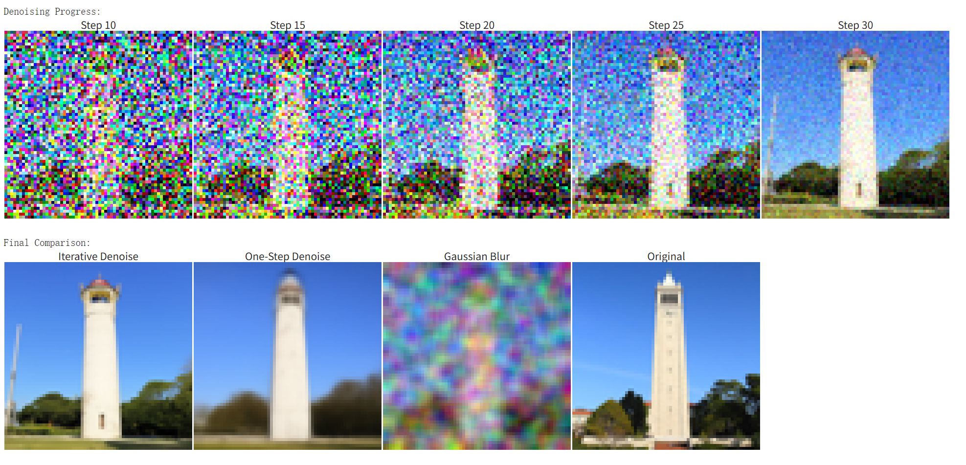
Part 1.5: Diffusion Model Sampling
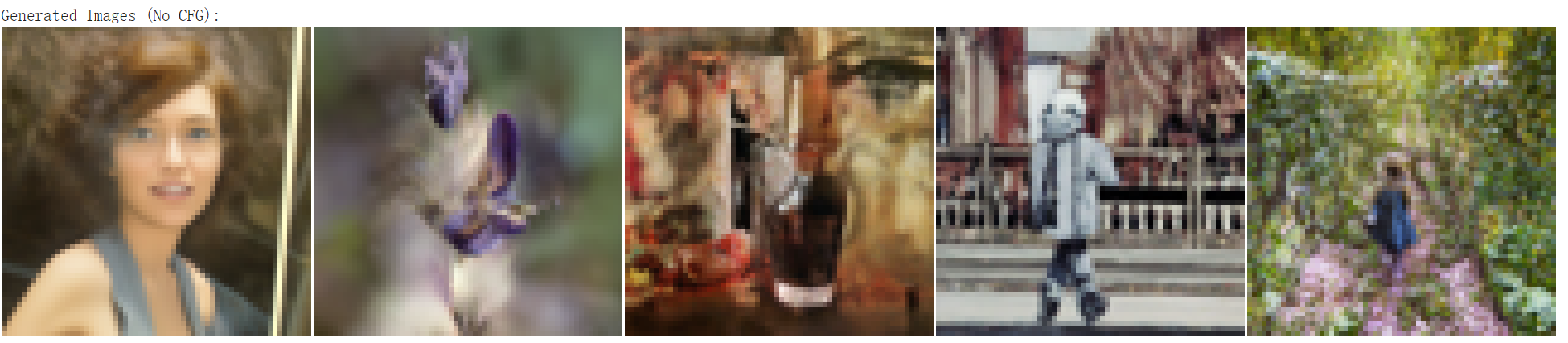
This part simply generates samples from pure noise and prompt "a high quality photo" using the diffusion model sampling loop.
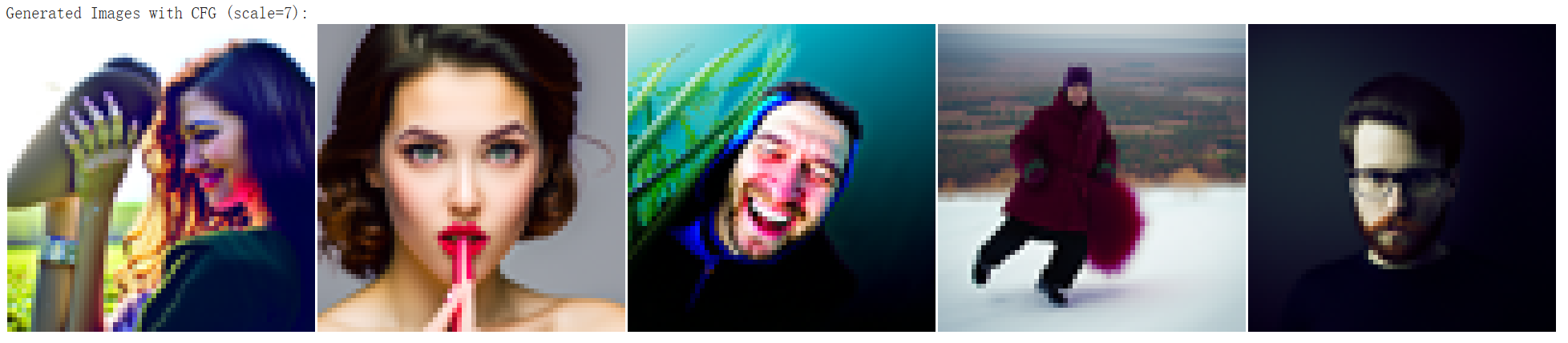
Part 1.6: Classifier-Free Guidance(CFG)
- Implement the
iterative_denoising_cfgfunction:
1 | |
- Results:
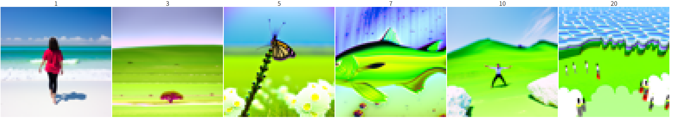
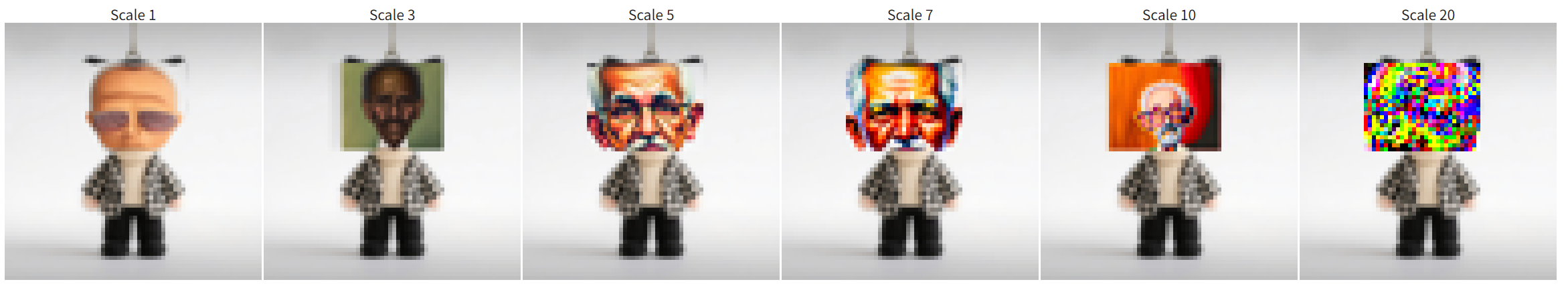
Part 1.7.1: Image-to-Image Translation
for web image:
- Original image:

- SDEdit result (for noise levels [1, 3, 5, 7, 10, 20] ):
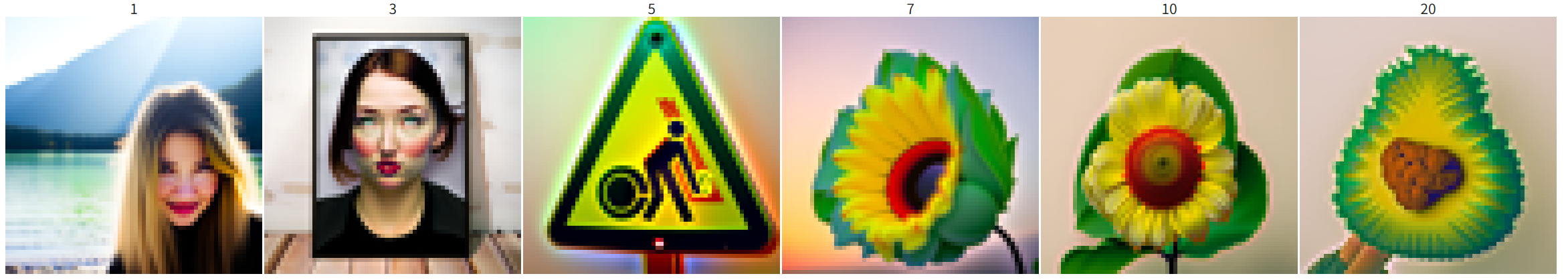
- Original image:
for handdrawn image 1:
- Original image:

- SDEdit result (for noise levels [1, 3, 5, 7, 10, 20] ):
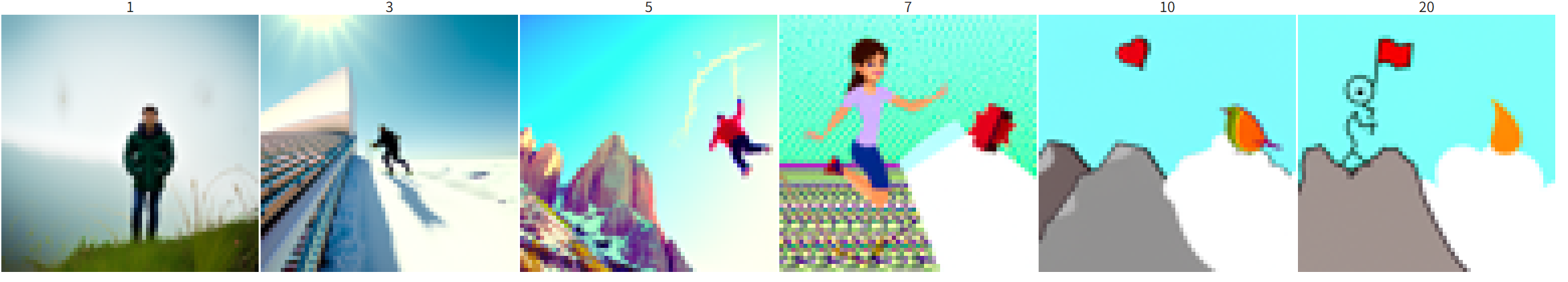
- Original image:
for handdrawn image 2:
- Original image:
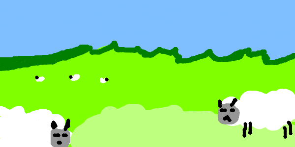
- SDEdit result (for noise levels [1, 3, 5, 7, 10, 20] ):
- Original image:
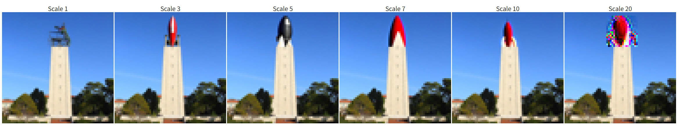
Part 1.7.2 & 1.7.3: Inpainting
Original image and mask:
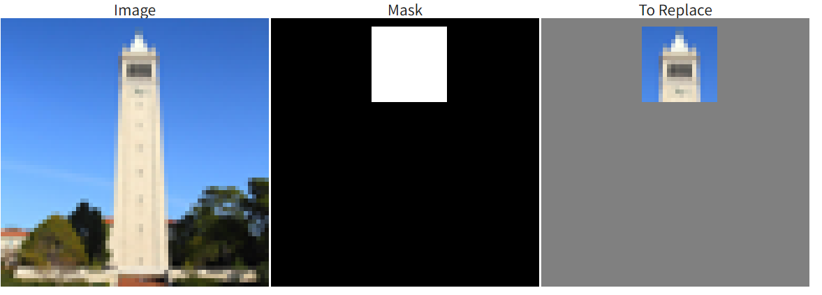
Replace the region with "a rocket ship" prompt:
Original image and mask:
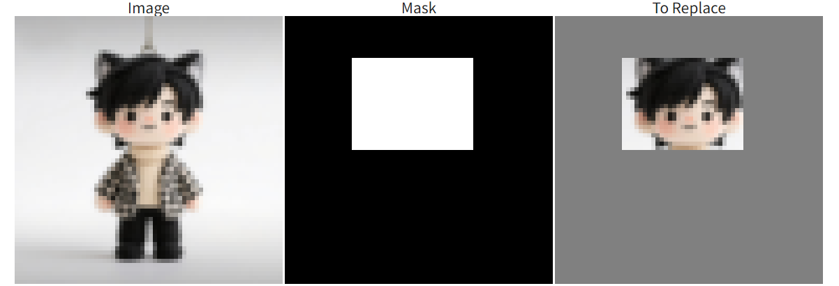
Replace the region with "an oil painting of an old man" prompt:
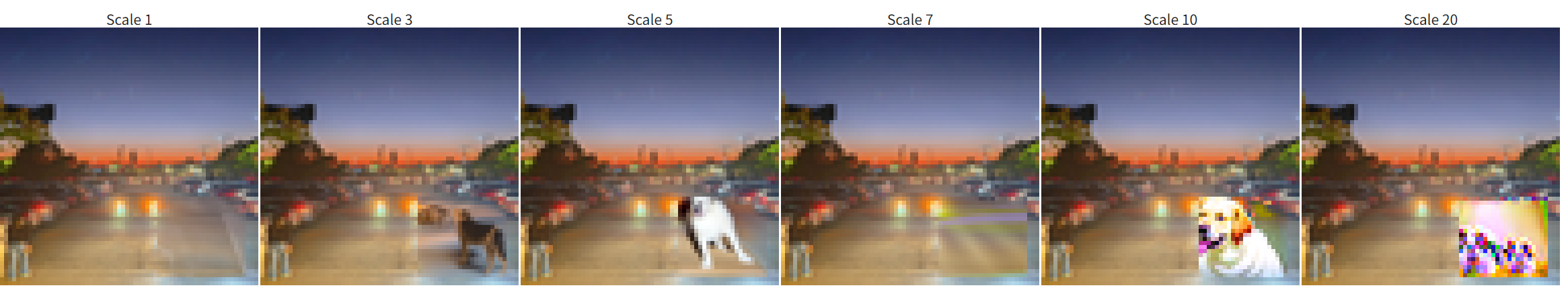
Original image and mask:
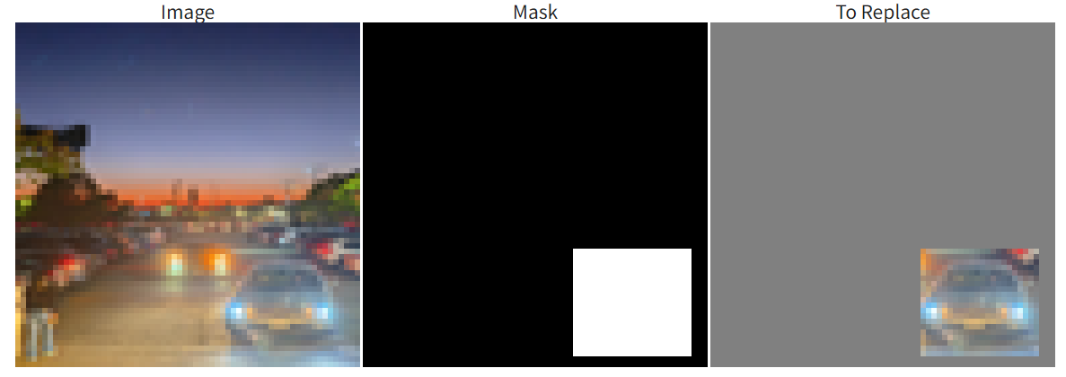
Replace the region with "a photo of a dog" prompt:
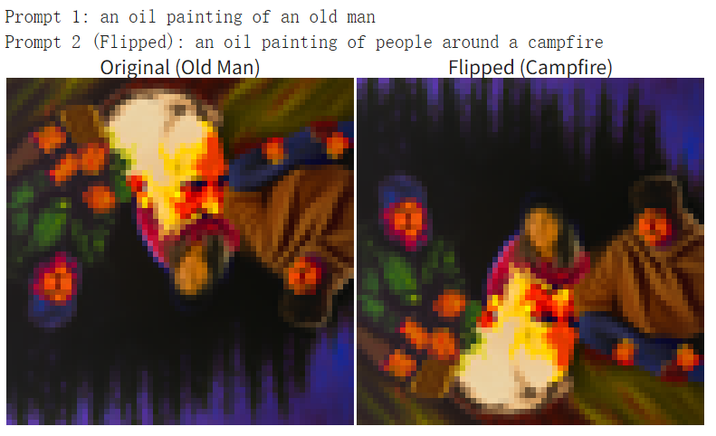
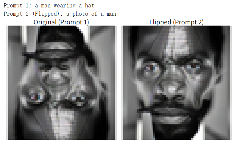
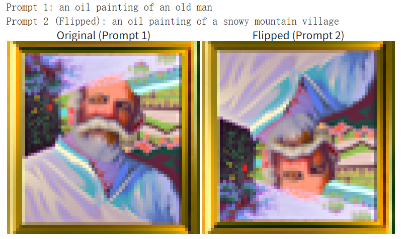
Part 1.8: Visual Anagrams
- Results:
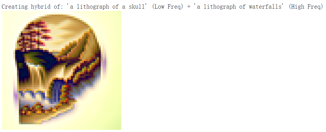
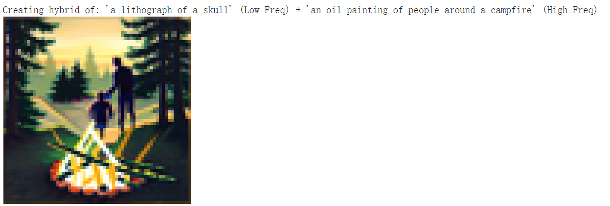
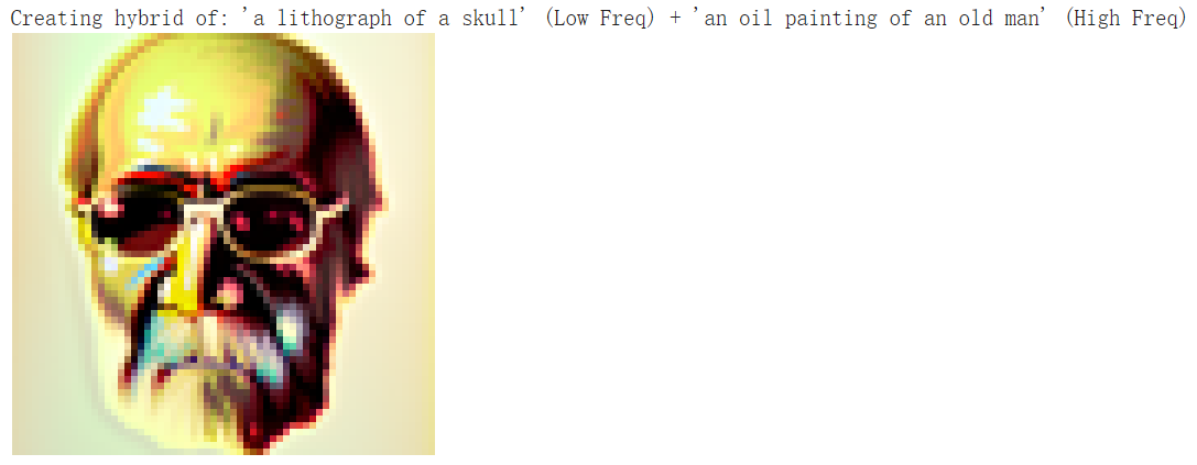
Part 1.9: Hybrid Images
The skull litograph is really suitable for low frequency part cause it is easy to recognize the skull shape even with low details.
- Results:
Deliverable (Part B)
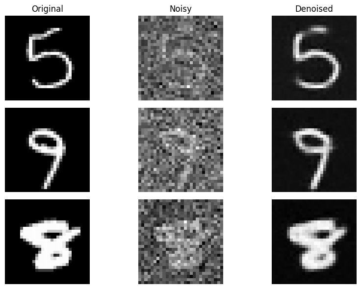
Part 1.1 & 1.2 Using the UNet to Train a Denoiser
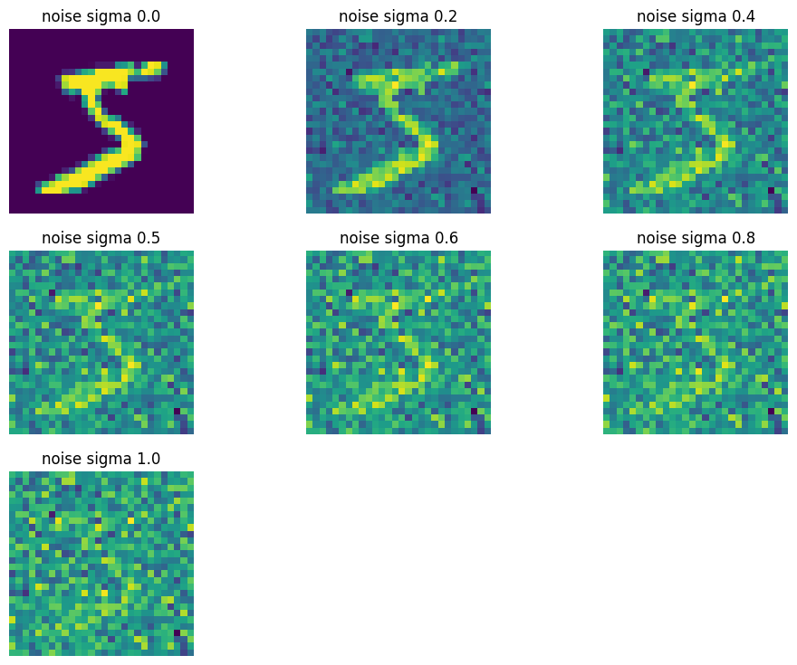
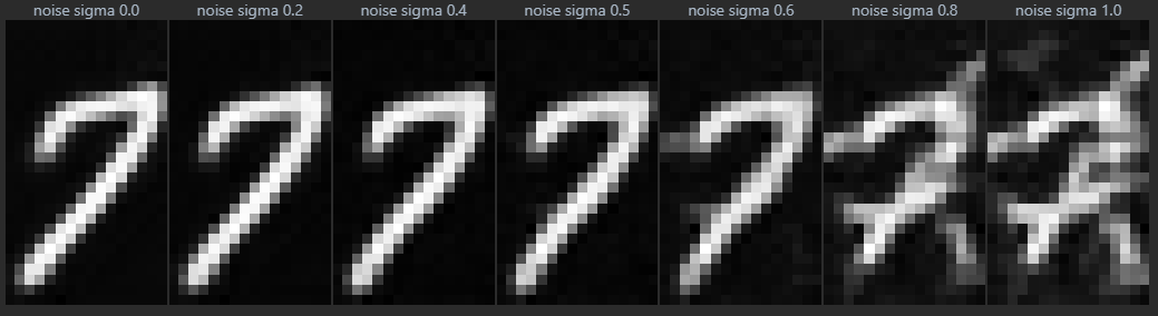
A visualization of the noising process using \(\sigma=[0.0, 0.2, 0.4, 0.5, 0.6, 0.8, 1.0]\)
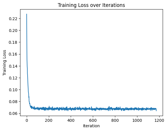
Part 1.2.1 Training (Unconditional, \(\sigma=0.5\))
After 1 epoch:
After 5 epoch:
Part 1.2.2 Out-of-Distribution Testing
test on \(\sigma=0.0, 0.2, 0.4, 0.5, 0.6, 0.8, 1.0\):
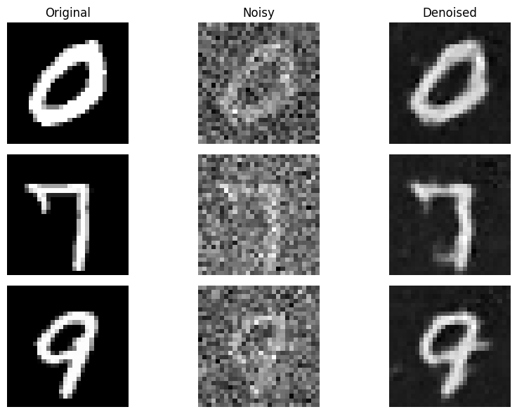
Part 1.2.3 Denoising Pure Noise
This time we start from pure noise and use the trained denoiser to iteratively denoise it.
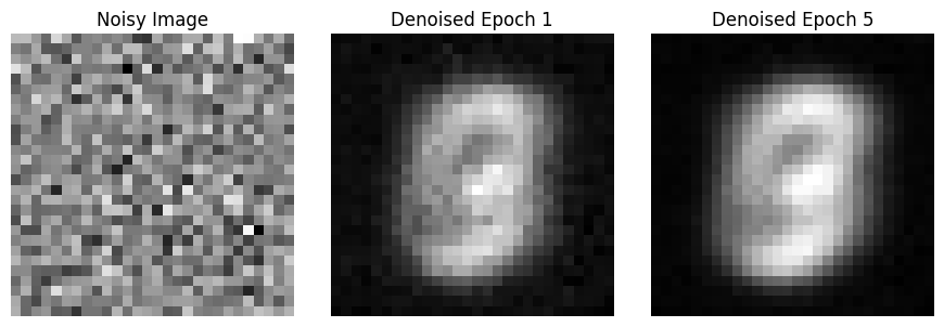
The final denoised image looks like the average of all digits, since the model is trained to denoise from various noisy images of different digits, so when starting from pure noise, it cannot figure out which digit to generate, thus generates an average digit.
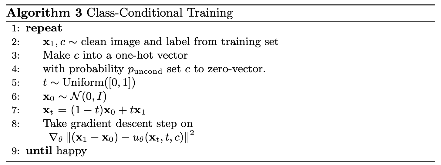
Part 2.1 & 2.2: Adding Time Conditioning to UNet & Training (Time-Conditioned)
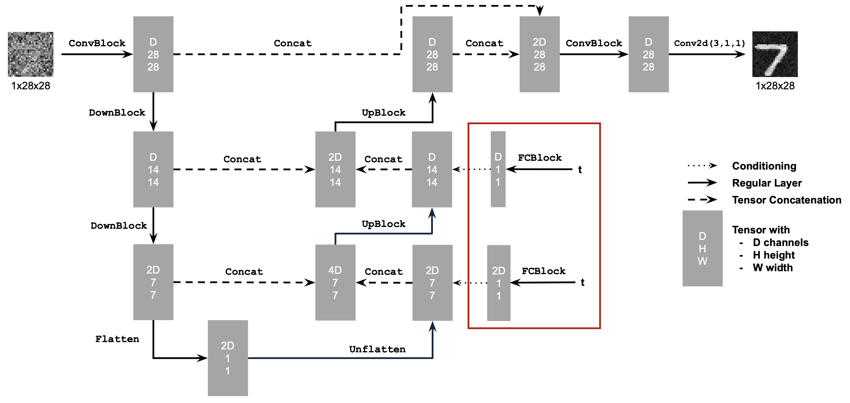
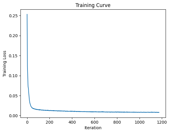
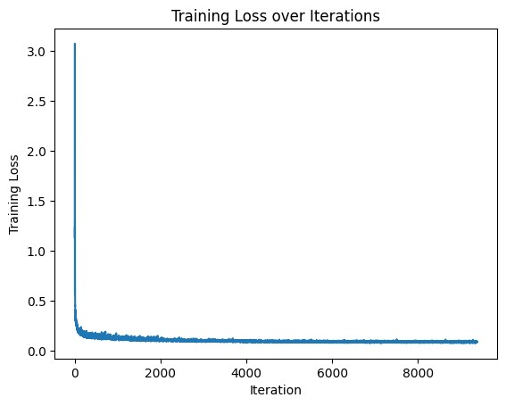
loss curve during training:
Part 2.3: Sampling from the UNet
Part 2.4 & 2.5: Adding Class-Conditioning to UNet & Training (Class-Conditioned)
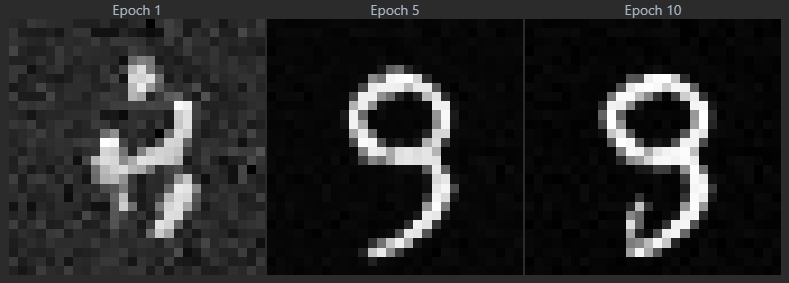
Part 2.6: Class-Conditioned Sampling from the UNet

epoch 1 animation:

epoch 5 animation:

epoch 10 animation:
If we remove the scheduler and just use a constant learning rate, the loss curve looks like this:
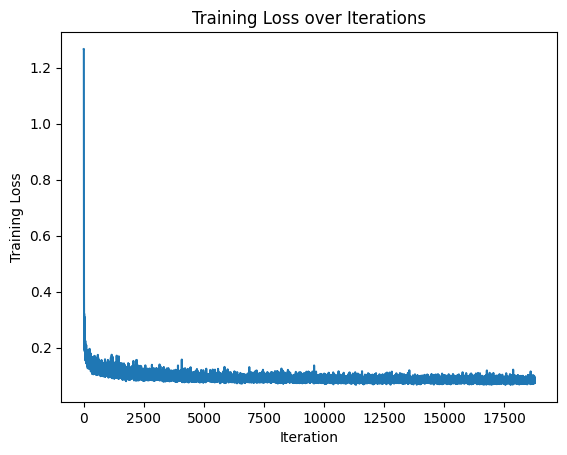
To get a similar result, I use a smaller learning rate of 3e-3 and
train for 15 epochs: 
epoch 1 animation:

epoch 5 animation:

epoch 10 animation:
