CS180-Proj4-NeRF

CS180 project4: NeRF

Theoretical Background

What is NeRF(Neural Radiance Fields)?

NeRF (proposed in the original 2020 paper) is the technique to represent a 3D scene volumetrically (i.e., without any surfaces) as a function parametrized by a neural network to render 2D views of such a scene and to train the network on a set 2D views.

Some reference tutorials about NeRF:

Functional Representation in 2D

How to represent a 2D image on a computer? There are several ways:

Functional Representation in 2D Representation of 2D images: a) – pixels , b) – vector, c) – point cloud, d) – functional

Is this all? No, there are more ways to represent an image mathematically. Let’s look at functional representations (sometimes also called implicit). There are several ways to use mathematical functions. First, we can parametrize the color C of a point \((x, y)\) as a mathematical function \(C = f(x, y)\). This is a volumetric representation for a 2D volume; it does not deal with any lines or curves (which are surfaces in 2D). On the other hand, we can have a surface representation \(f(x,y) = 0\), a contour parametrized by an implicit function.

But how can we represent a complicated nonlinear function \(f(x, y)\) on the computer? In 2025 we all know the answer: deep neural networks. There is an experiment that probably every person really interested in deep learning has tried at least once: approximate the function \(C=f(x, y)\) with a fully-connected neural network (also known as a multi-layer perceptron or MLP) and train it on all pixels of an image. The dataset here consists of tuples \((x, y, C)\) for all image pixels of a single image. Once trained, we use this MLP to predict the color C for all pixels \((x, y)\), and thus we use \(f(x, y)\) to render an image. This part is exactly what we will implement in Part 1. But let's see how this naive approach works:

(From left to right illustrates the network output at 0, 100, 300, 800, 1500 and 3000 training iterations)

It’s not particularly good, despite the neural network having more parameters than pixels in the image, why? This representation has two problems:

The raw coordinates \((x, y)\) are not a good input representation for the neural network. The network cannot easily learn high-frequency functions from such inputs. So the solution is to use positional encoding (Fourier features) to map the input coordinates \((x, y)\) to a higher-dimensional space with more frequency components. This is what we will implement in Part 1.
The ReLU-based MLPs can only represent piecewise linear functions. More sophisticated activation functions (e.g. Sigmoid, Sine) or network architectures (e.g. SIREN, Fourier Neural Operator) can help to represent high-frequency functions better.

This is the better result after applying positional encoding and sigmoid activation:

Functional Representation in 3D: TSDF and NeRF

How to represent 3D objects digitally? 3D representations follow the same ideas as 2D ones.

Pixels in 3D become voxels. Point cloud in 3D is defined just like in 2D. Polygonal meshes can be viewed as a special case of vector graphics. What about the functional representation? Once again, we have two types of it: surface and volumetric.

Surface functional representation is about describing the surfaces with the implicit equation \(f(x, y, z) = 0\). This family of methods is called the (truncated) signed distance function or (T)SDF. The volumetric representation is given by the formula \(C=f(x, y, z)\), giving the color \(C\) of each 3D point \((x, y, z)\). We can think of these as “continuous voxels” or 3D translucent object made of colored jelly.

This is basically what NeRF is, although in order to achieve better results, the actual NeRF adds two things: directional dependence and density.

NeRF Theory

There are three main components of NeRF: scene representation, renderer and the training regime. NeRF represents a 3D scene as a 5D function parametrized by a neural network:

The inputs are the coordinates \(r=(x, y, z)\) and the viewing direction \((\theta, \phi)\), often replaced by a unit direction vector \(d=(d_1, d_2, d_3)\). The actual inputs to the MLP are the positional encodings of these two vectors. The output is the color \(C=(r, g, b)\) and the density \(\sigma\).

But what about the lighting? The “standard” NeRF makes the following strict assumptions about the lighting:

every point in the 3D scene emits light equally in all directions (i.e., no specular reflections);
every point in the 3D scene absorbs light according to its density \(\Sigma\) only (i.e., no subsurface scattering).

As a result, the lighting conditions of the scene are frozen and cannot be changed after training.

Differentiable Volume Rendering

As we cannot perceive a 3D scene directly, what we typically want is to render it from a certain viewpoint or view, specified by the camera parameters: intrinsic (focal length, image size) and extrinsic (camera position and direction). The result is a 2D image. Each camera pixel becomes a ray in the 3D scene. The pixel color includes contributions from all points along the ray given by the sum (or rather integral, as our model is continuous) over the points along the ray:

\[ C(r) = \int_{t_n}^{t_f} T(t) \sigma(r(t)) c(r(t), d) dt, \]

where \(r(t) = o + t d\) is the point along the ray at distance \(t\) from the camera center \(o\) in direction \(d\), \(c(r(t), d)\) is the color at point \(r(t)\) in direction \(d\), \(\sigma(r(t))\) is the density at point \(r(t)\), and \(T(t) = \exp(-\int_{t_n}^{t} \sigma(r(s)) ds)\) is the accumulated transmittance from \(t_n\) to \(t\). \(T(t)\) gives the fraction of the light intensity from the point t reaching the camera (the rest is absorbed). In the rendering slang it is also called “probability of the ray reaching the point t uninterrupted”.

In practice, NeRF uses a set of discrete points along the ray. For each point, get the \(c\) and \(\sigma\) from \(f(r(t), d)\), and then use sum to approximate the integral. However this would lead to a fixed set of 3D points, which could potentially lead to overfitting when we train the NeRF later on. On top of this, we want to introduce some small perturbation to the points only during training, so that every location along the ray would be touched upon during training. this can be achieved by something like t = t + (np.random.rand(t.shape) * t_width) where t is set to be the start of each interval.

Deliverables

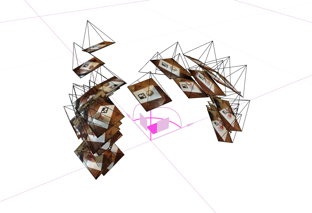
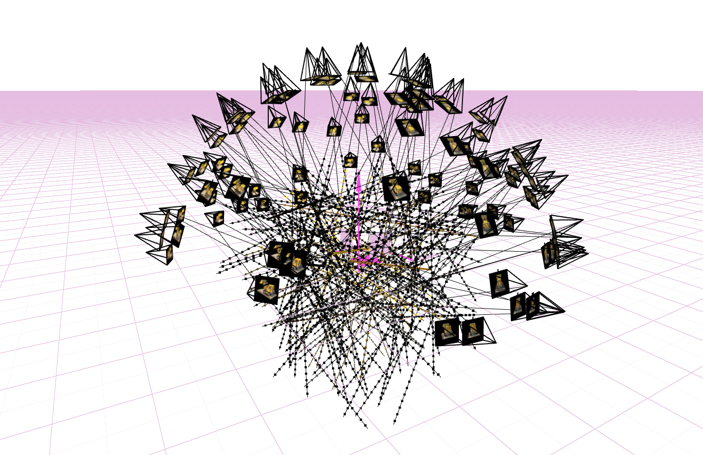
Camera Calibration and 3D Scanning
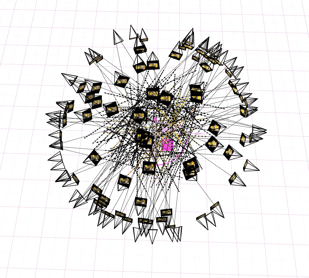
- 3 screenshots of your camera frustums visualization in Viser:
Fit a Neural Field to a 2D Image
- Model architecture report (number of layers, width, learning rate, and other important details) "num_freqs": 10, "hidden_dim": 256, "num_layers": 3, "learning_rate": 0.01, "iterations": 3000, "batch_size": 10000,
- Training progression visualization on both the provided test image and one of your own images
- Final results for 2 choices of max positional encoding frequency and 2 choices of width (2x2 grid)
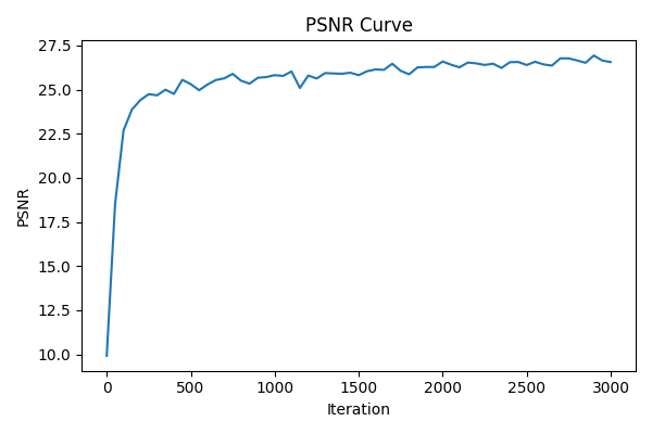
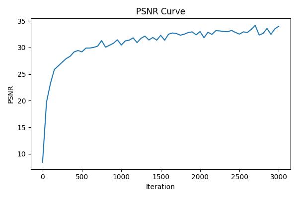
- PSNR curve for training on one image of your choice
  - on the provided test image
  - on my own image

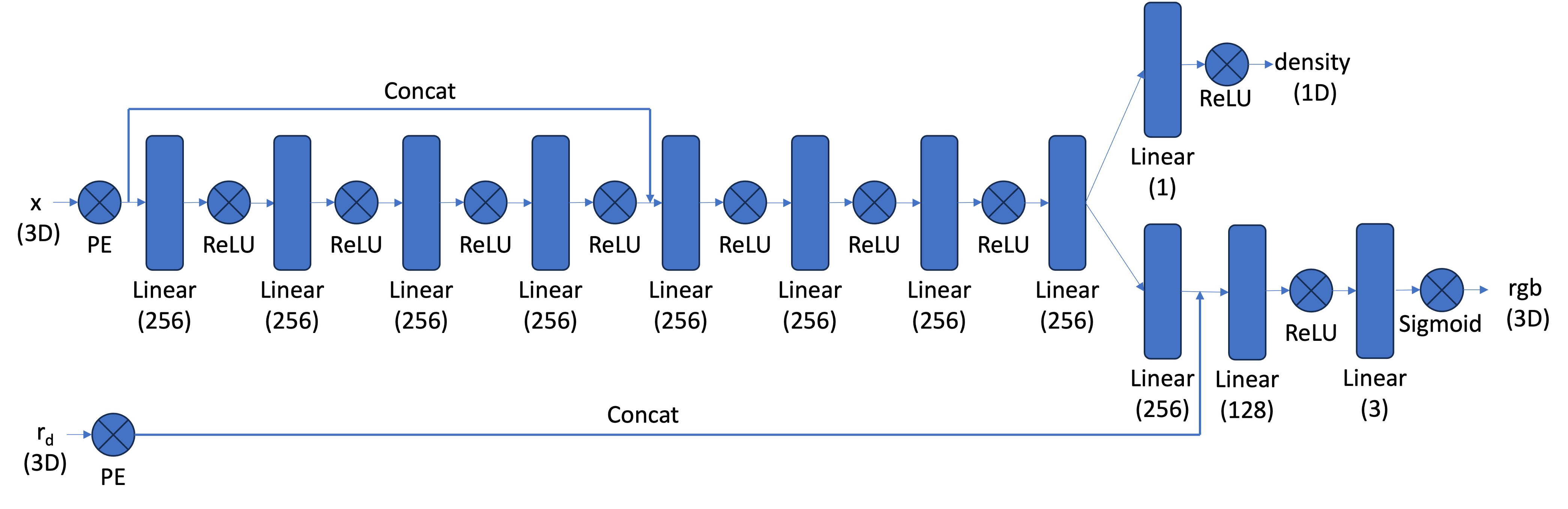
Fit a Neural Radiance Field from Multi-view Images

Implementation details (Pseudocodes)

Create Rays from Cameras

def transform(c2w, x_c):
    # to transform camera coordinates to world coordinates
    x_w = c2w @ x_c
    return x_w

def pixel_to_camera(K, uv, s):
    # to transform pixel coordinates to camera coordinates
    # K: intrinsic matrix, uv: pixel coordinates, s: depth
    fx, fy, cx, cy = K[0, 0], K[1, 1], K[0, 2], K[1, 2]
    u,v = uv[:,0], uv[:,1]
    x = (u - cx) * s / fx
    y = (v - cy) * s / fy
    z = s * np.ones_like(u)
    return np.stack([x, y, z], axis=-1)

def pixel_to_ray(K, c2w, uv):
   # Convert pixel coordinates to a ray (origin + normalized direction) in world space.
   point_camera = pixel_to_camera(K, uv, s=1.0)  # assume depth s=1.0
   point_world = transform(c2w, point_camera.T).T
   ray_origin = point_world
   ray_direction = point_world - c2w[:3, 3]
   ray_direction /= np.linalg.norm(ray_direction) # normalize
   return ray_origin, ray_direction

NeRF Network Structure

Rays Visualization
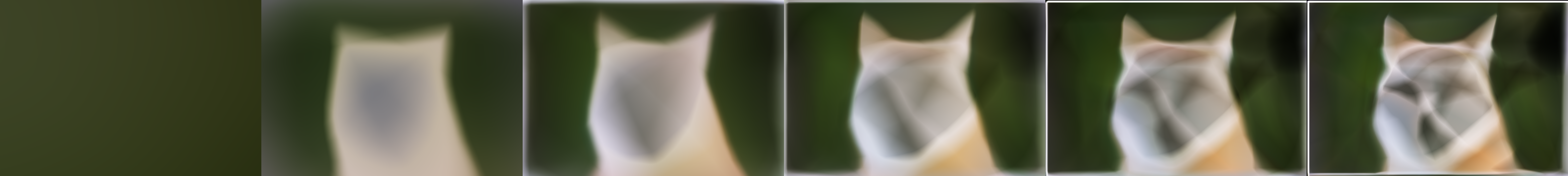
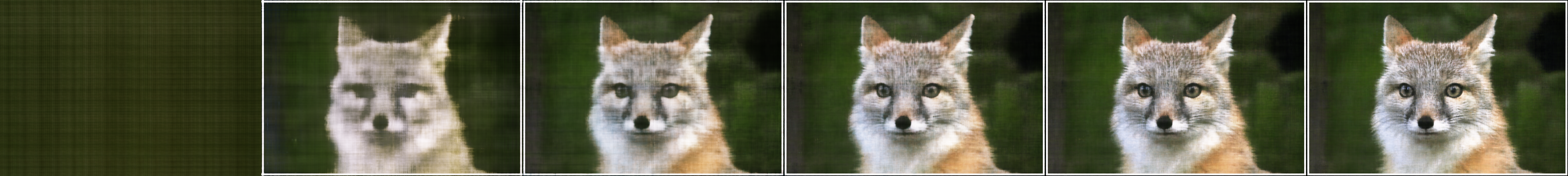
Training progression visualization (rendered images at different training iterations)

Iteration Dataset Rendered Image

1000 Lego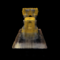

3000 Lego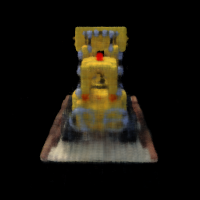

5000 Lego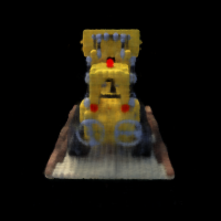

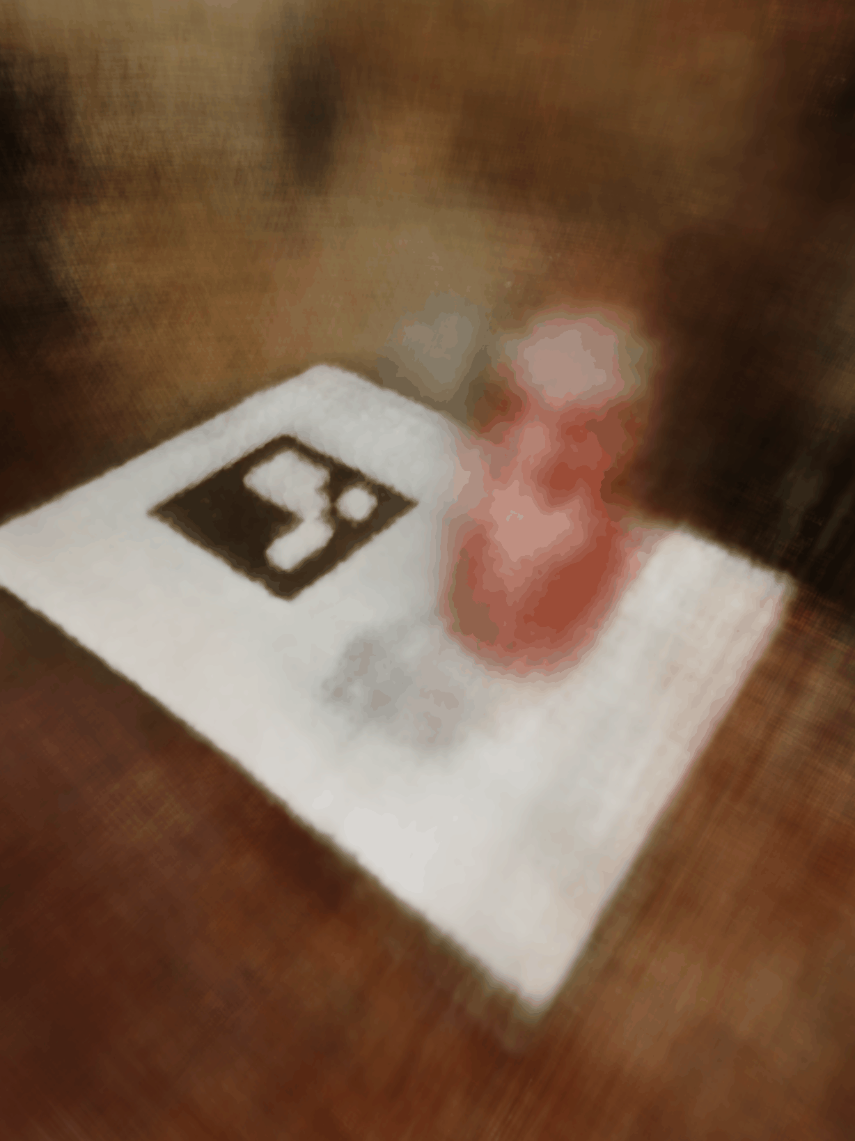
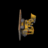
300 My Data

1500 My Data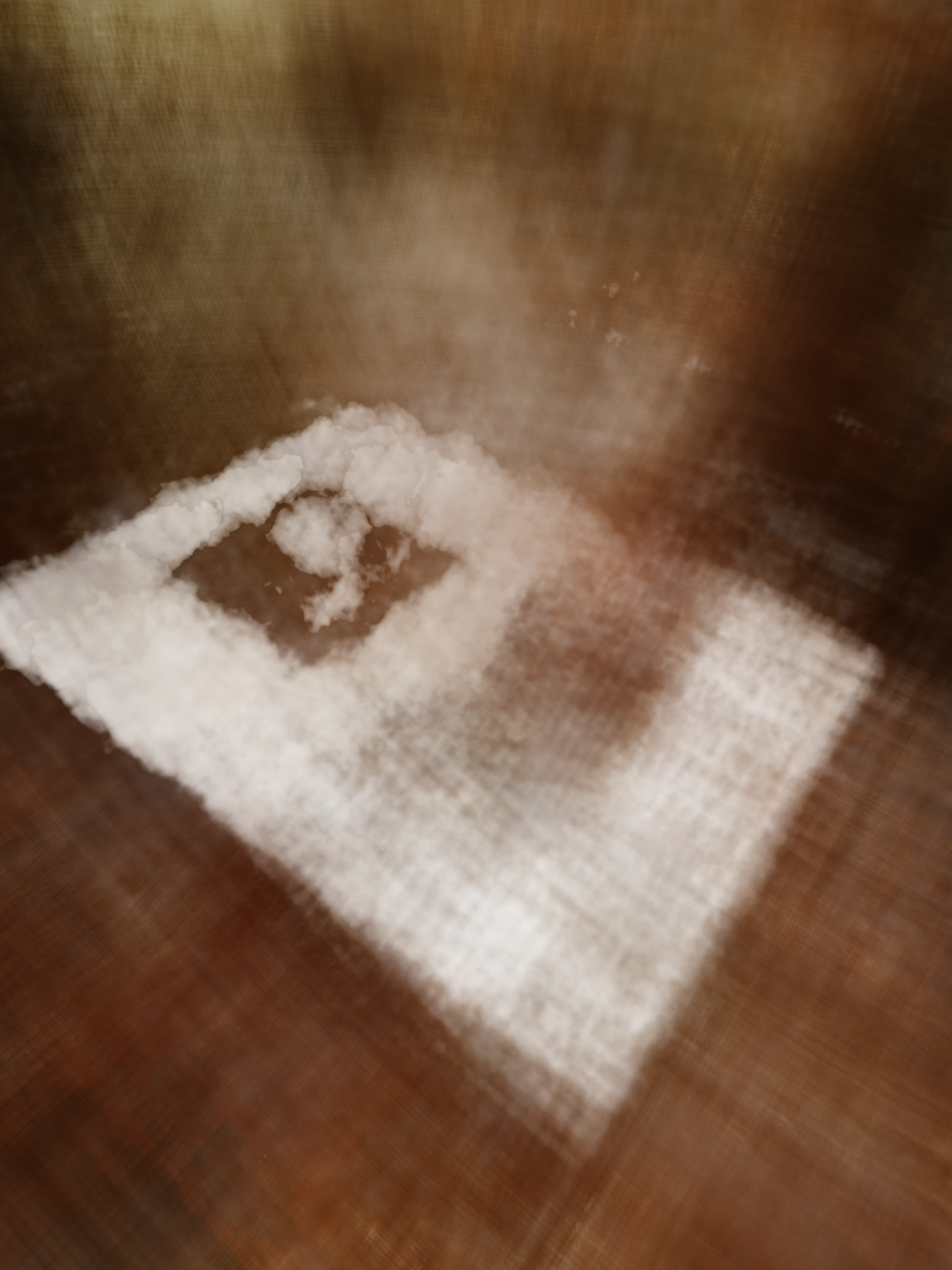

5000 My Data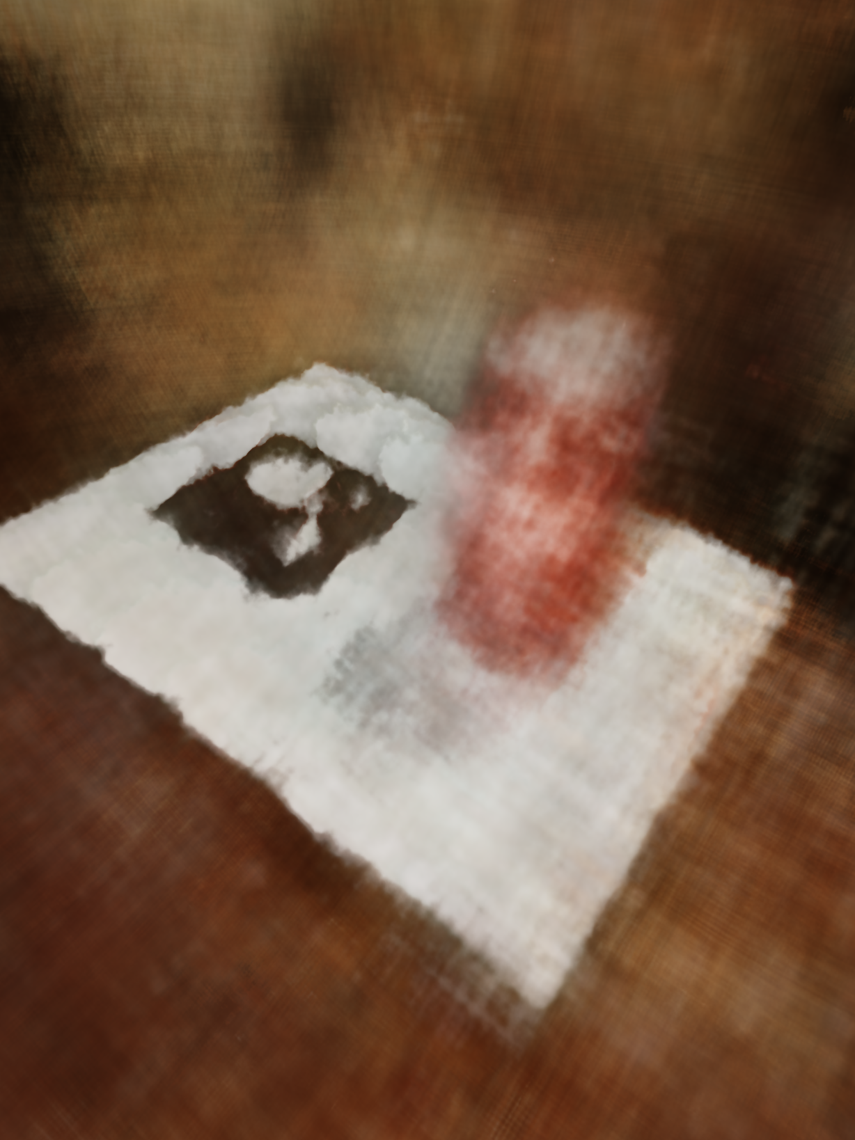
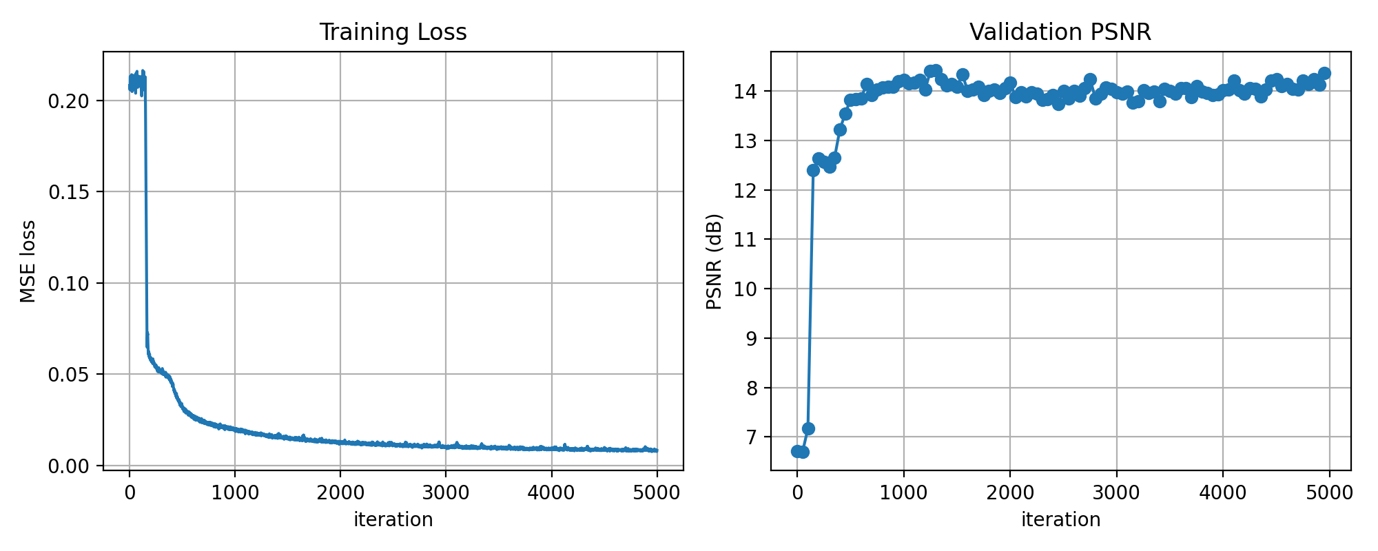
PSNR and Loss curves during training
- on the provided lego dataset
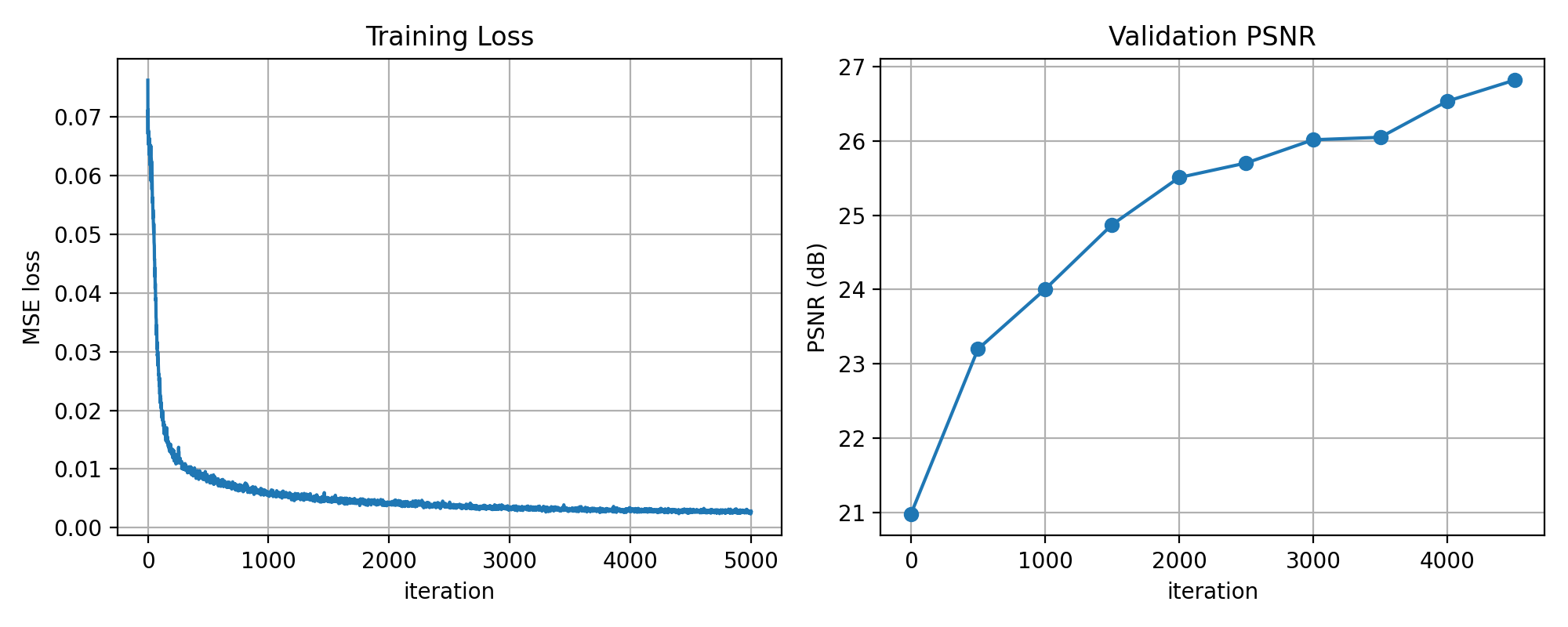
- on my own dataset
Final rendered GIFs
- on the provided lego dataset (batch = 8192, iterations = 5000)
- on my own dataset (batch = 8192, sample =128, iterations = 5000)