CS180-Proj3A

CS180 Lab 3 - Part A

Overview

It's trivial for us to do several types of geometric transformations: translation, rotation, scaling, skewing, etc. They can all be represented as matrix multiplications. However, when we want to stitch two or more images from different viewpoints together, we need to use a more general transformation called homography.

Some math

Homography

From Wikipedia:

In the field of computer vision, any two images of the same planar surface in space are related by a homography (assuming a pinhole camera model).

Homography

The homography is a function \(h\) that maps points into points, with the property that if points \(x\), \(y\), and \(z\) are colinear, then the transformed points \(h(x)\), \(h(y)\), and \(h(z)\) are also colinear. So the function \(h\) can be represented as a matrix multiplication:

\[ \begin{bmatrix} x'/w' \\ y'/w' \\ 1 \end{bmatrix} \longleftrightarrow \begin{bmatrix} x' \\ y' \\ w' \end{bmatrix} = H \begin{bmatrix} x \\ y \\ 1 \end{bmatrix} \]

where \(H\) is a 3x3 matrix, and \((x', y', w')\) are the transformed coordinates in homogeneous coordinates.

How to compute H?

First, we suppose H is:

\[ H = \begin{bmatrix} h_{11} & h_{12} & h_{13} \\ h_{21} & h_{22} & h_{23} \\ h_{31} & h_{32} & h_{33} \end{bmatrix} \]

Then we assume we have \(n\) pairs of corresponding points \((x_i, y_i)\) and \((x'_i, y'_i)\), where \(i = 1, 2, ..., n\). Each pair gives us two equations:

\[ x'_i = \frac{h_{11} x_i + h_{12} y_i + h_{13}}{h_{31} x_i + h_{32} y_i + h_{33}} \]

\[ y'_i = \frac{h_{21} x_i + h_{22} y_i + h_{23}}{h_{31} x_i + h_{32} y_i + h_{33}} \]

so we can define \(h\) as:

\[h = [h_{11}, h_{12}, h_{13}, h_{21}, h_{22}, h_{23}, h_{31}, h_{32}, h_{33}]^T\]

Thus, we can get a system of linear equations \(Ah = 0\), where \(A\) is a \(2n \times 9\) matrix below:

\[ A = \begin{bmatrix} x_1 & y_1 & 1 & 0 & 0 & 0 & -x'_1 x_1 & -x'_1 y_1 & -x'_1 \\ 0 & 0 & 0 & x_1 & y_1 & 1 & -y'_1 x_1 & -y'_1 y_1 & -y'_1 \\ \cdots & & & & & & & & \\ x_n & y_n & 1 & 0 & 0 & 0 & -x'_n x_n & -x'_n y_n & -x'_n \\ 0 & 0 & 0 & x_n & y_n & 1 & -y'_n x_n & -y'_n y_n & -y'_n \end{bmatrix} \]

And we can solve this by SVD. The solution is the right singular vector corresponding to the smallest singular value of \(A\). (Finally, we need to reshape \(h\) back to a 3x3 matrix \(H\).)

Also, from the above, we can see that we need at least 4 pairs of corresponding points to solve for \(H\). (every pair gives us 2 equations, and we have 8 degrees of freedom)

---

A.1 Shoot and Digitize Pictures

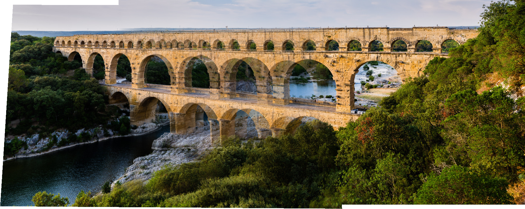
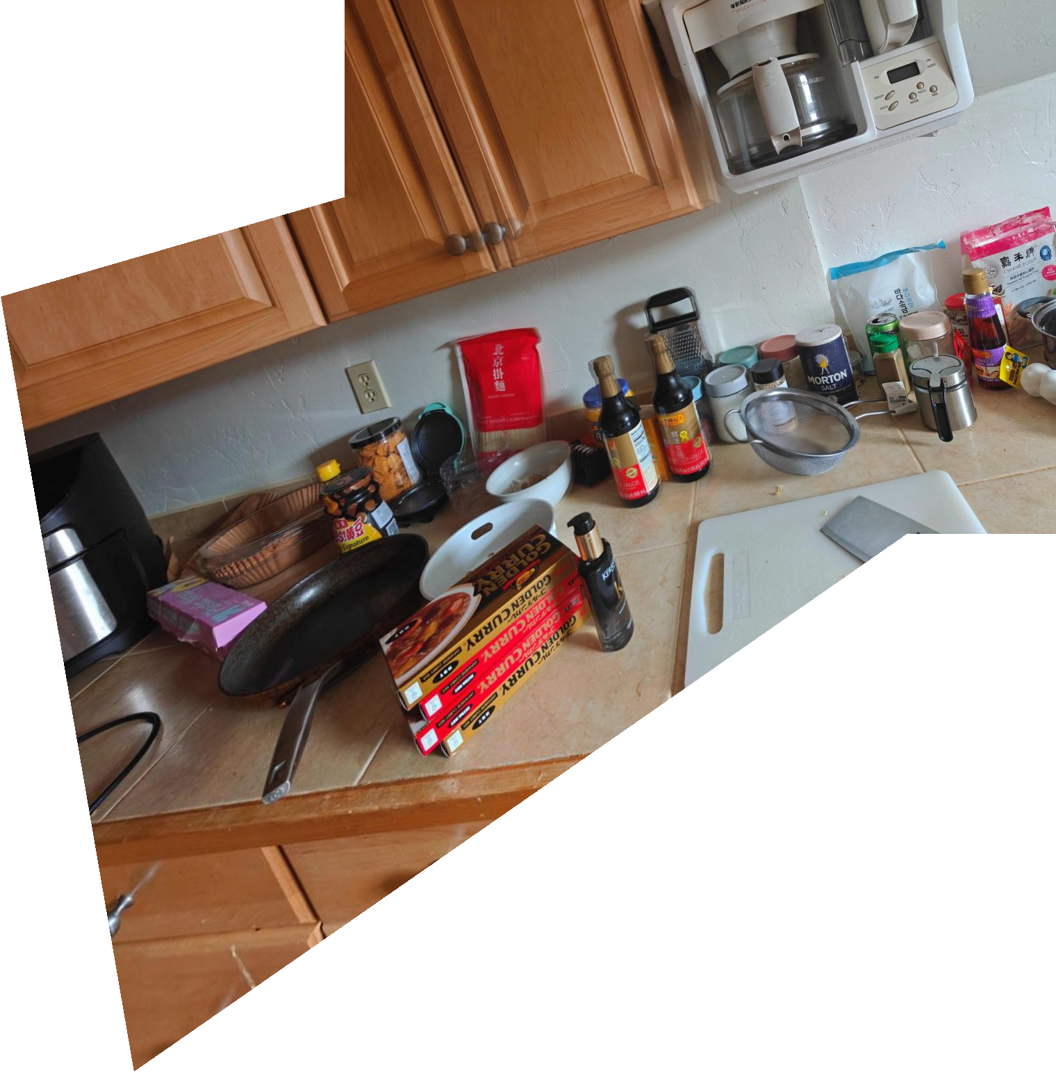
I prepared three image pairs with large planar overlap:

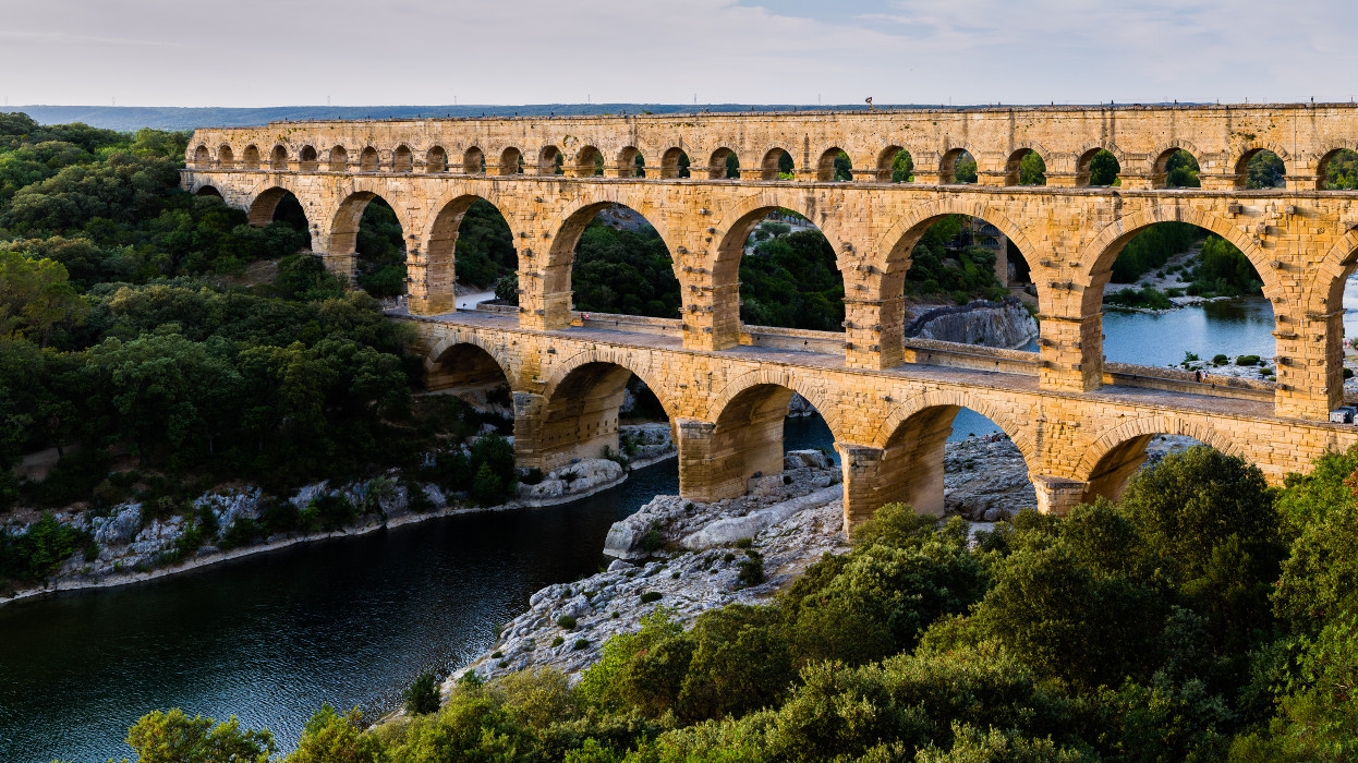
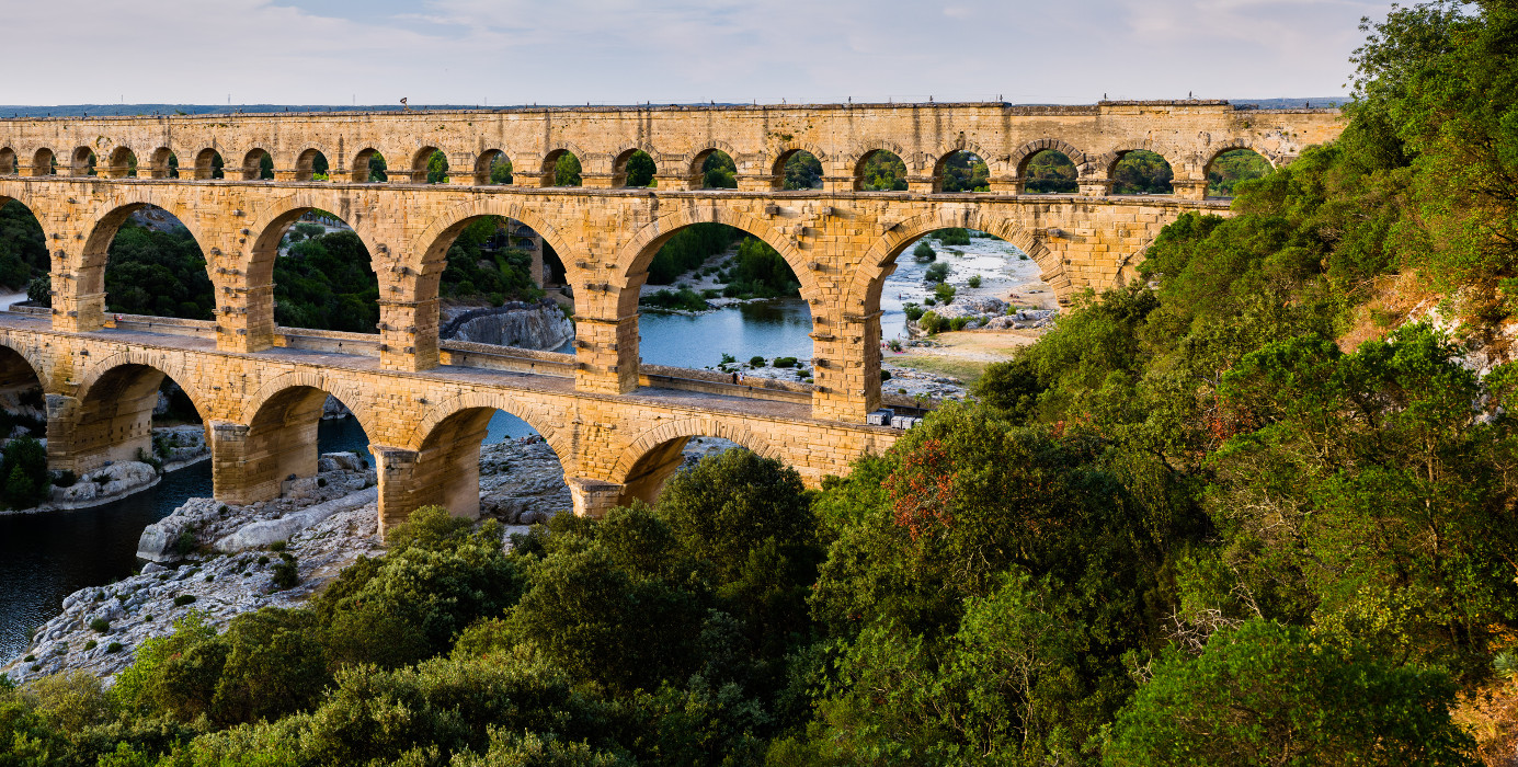
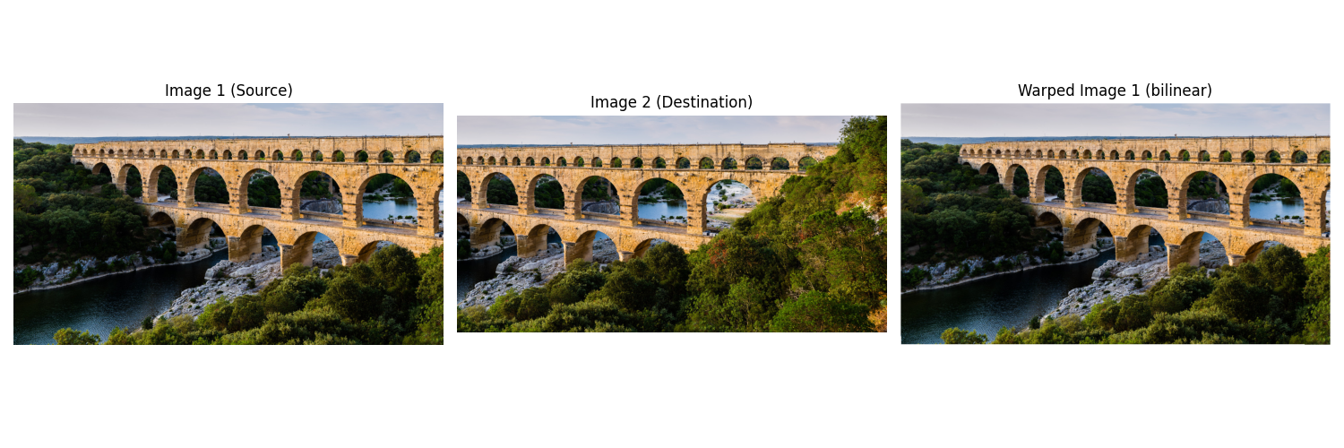
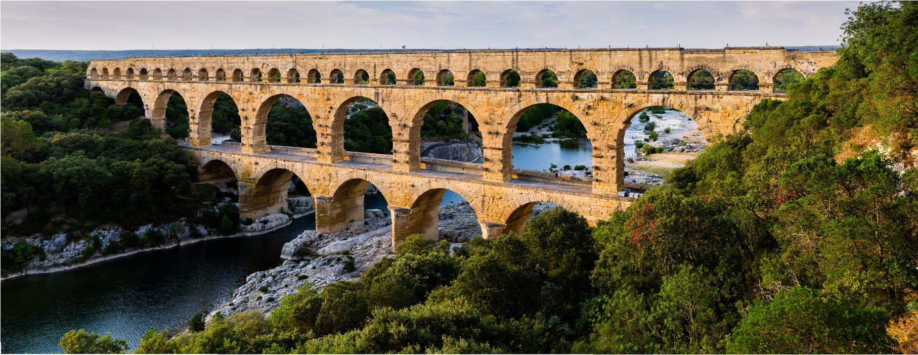
• Bridge: the provided OpenCV panorama example for a controlled baseline (panning around a riverside walkway).
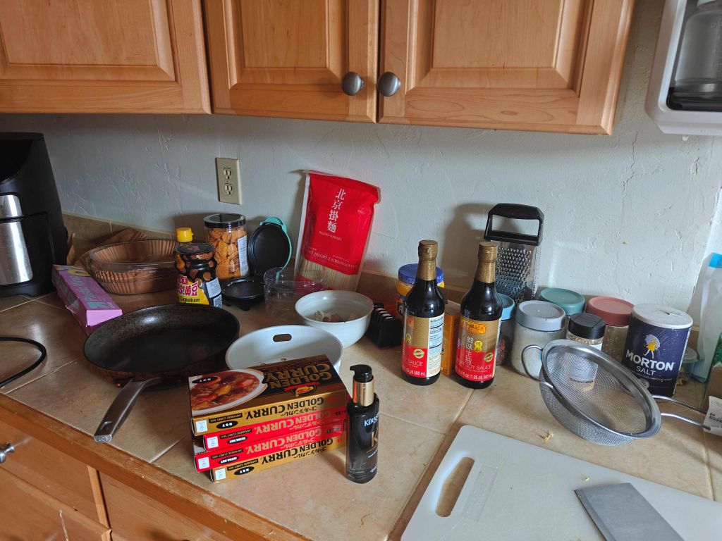
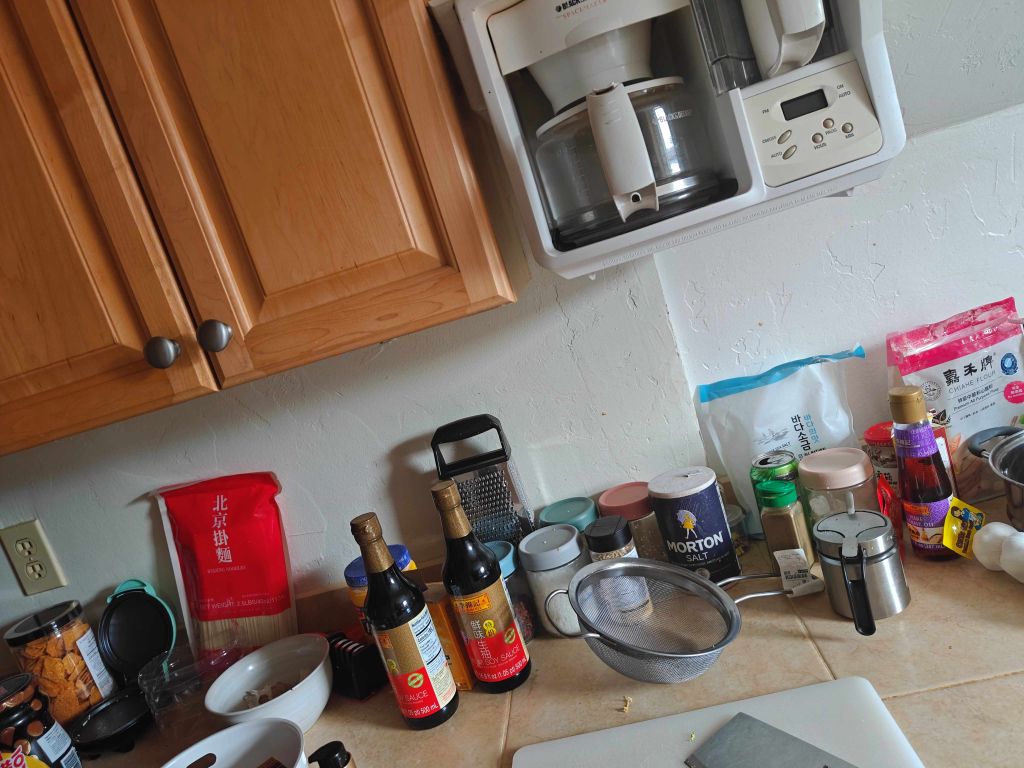
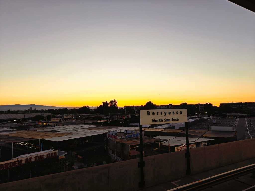
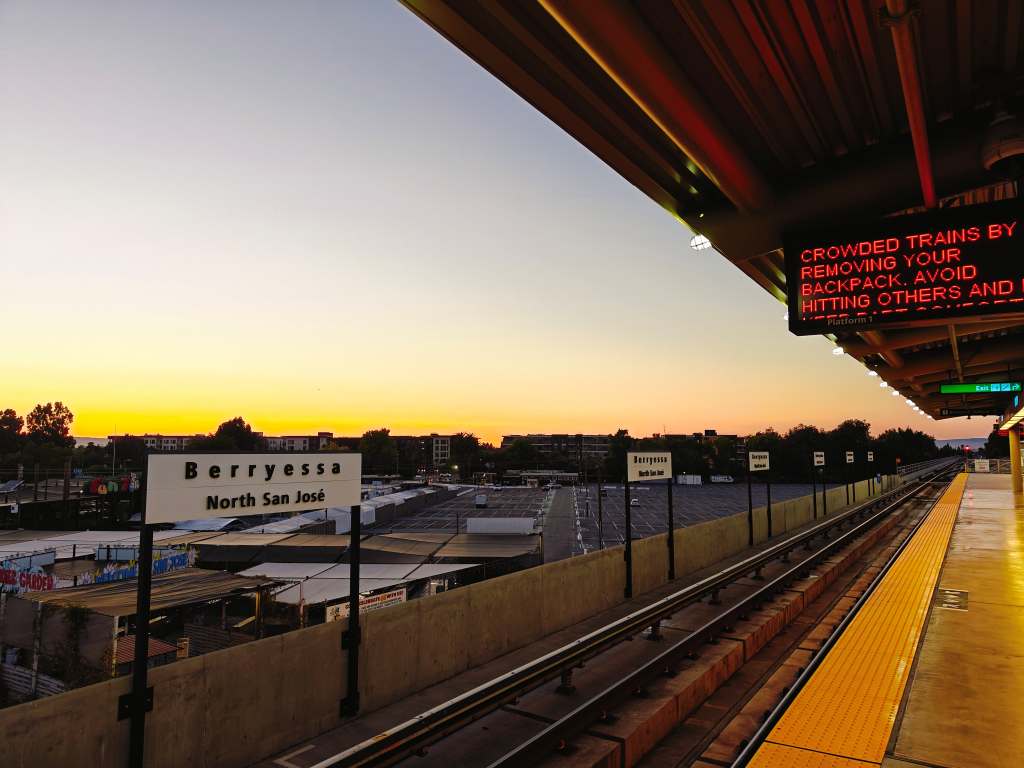
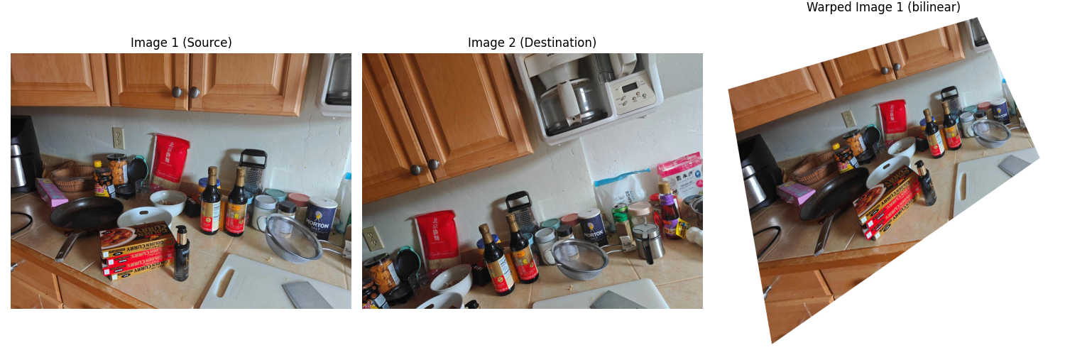
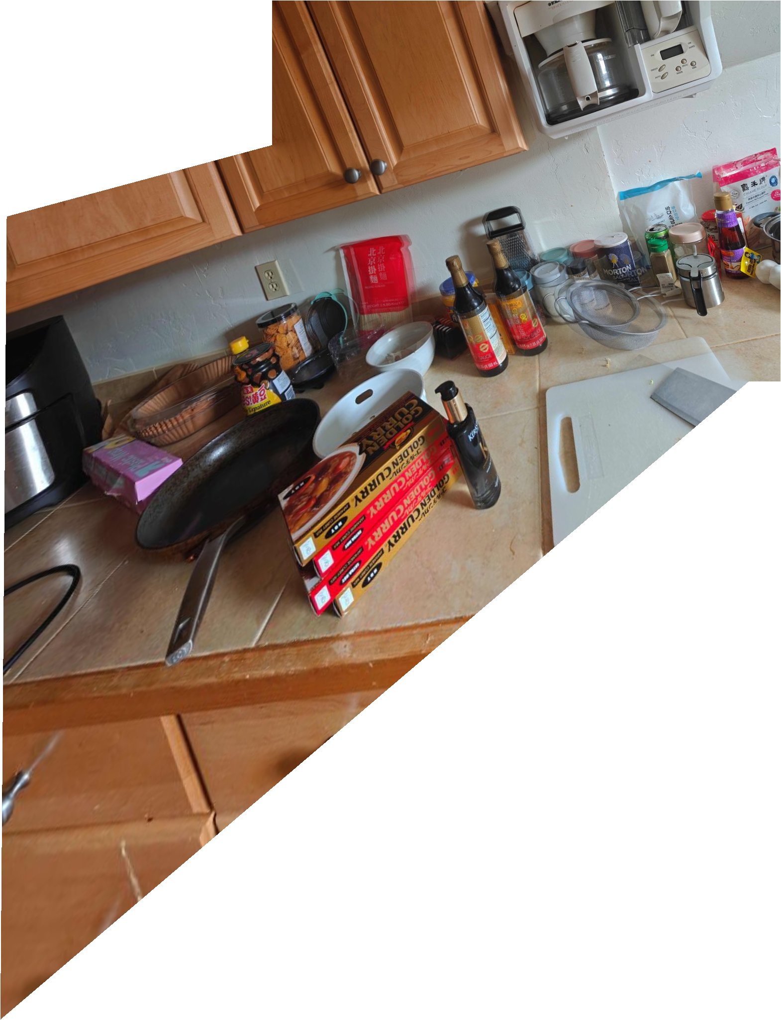
• Kitchen: two handheld shots of my kitchen counter taken a few inches apart while rotating the camera about the optical center.
• Table: a tabletop arrangement with books and a monitor, again acquired by pivoting the camera to keep the motion approximately projective.

Representative inputs are shown below (left/right are the two source images in each pair):

A.2 Recover Homographies

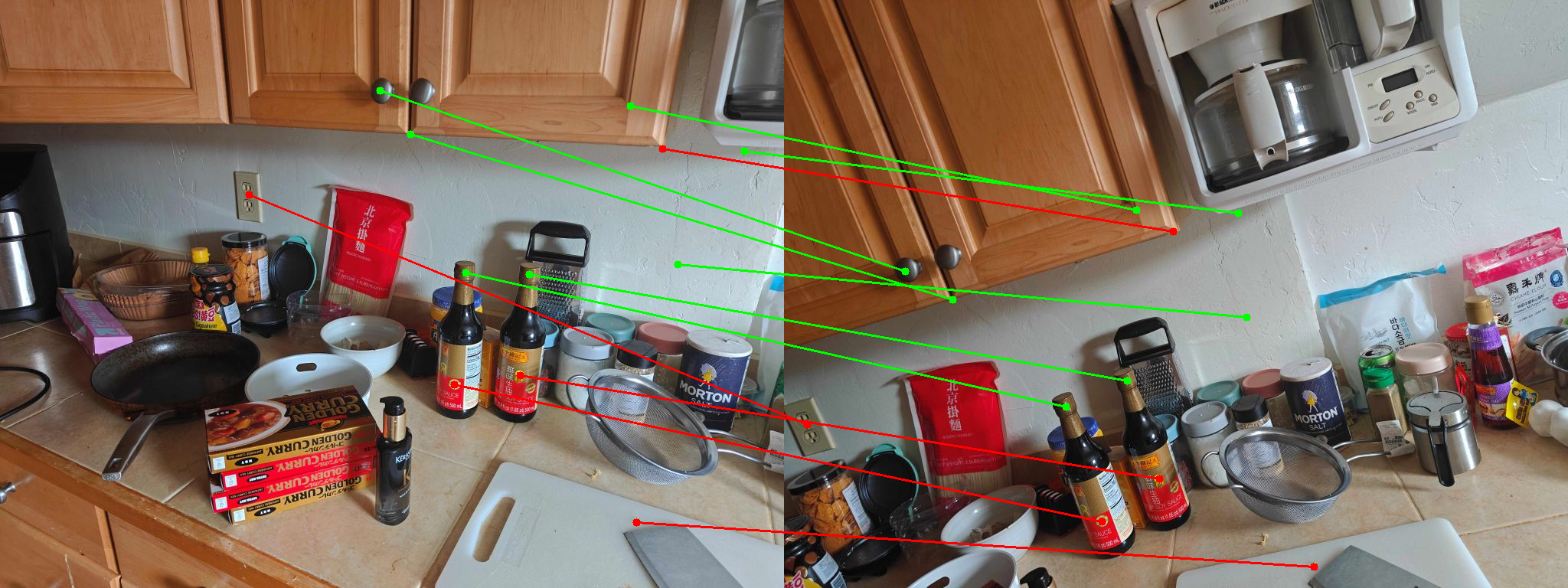
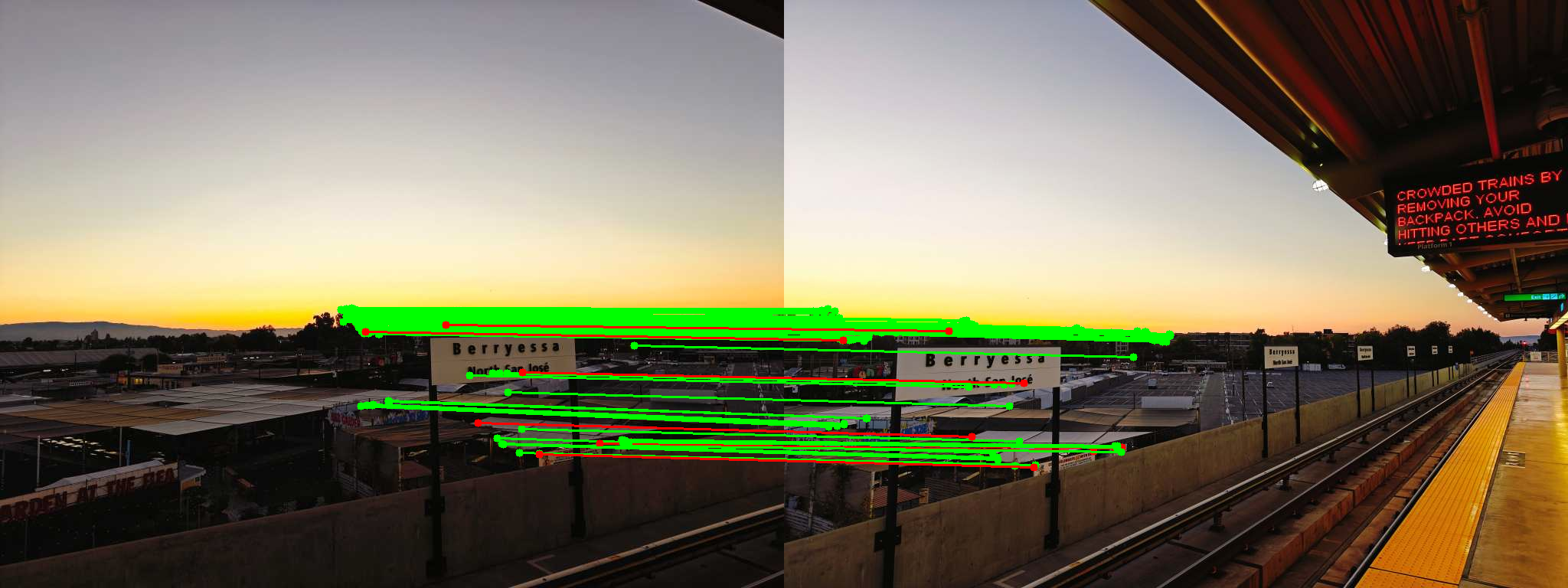
Correspondences come either from manual clicking (JSON files in test_data/.../*.json). The correspondence are shown below:

• Bridge:

• Kitchen:

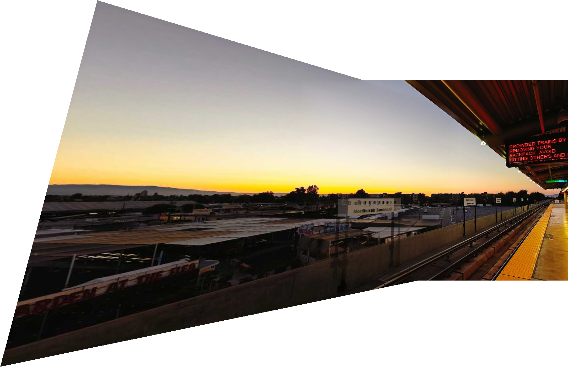
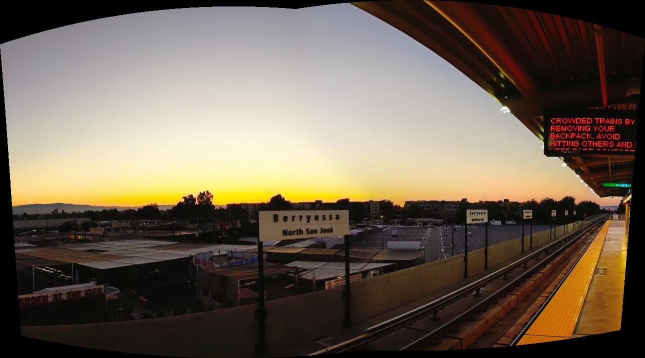
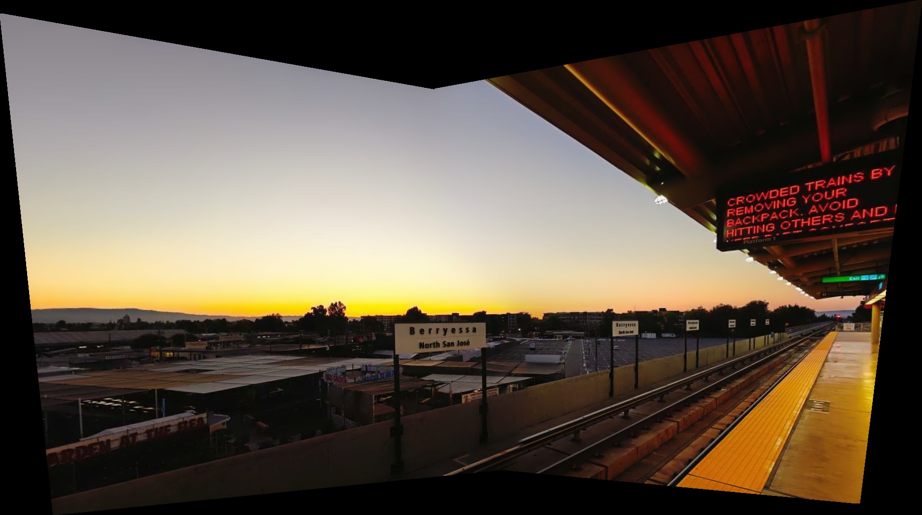
• Station:

The estimated homographies are:

\[ H_{bridge} = \begin{bmatrix} 1.000517151994700926e+00 & 1.934651821424284305e-05 & -4.292858059440893612e+02 \\ -1.347010553204711417e-04 & 1.000425656962335097e+00 & -1.110208515622688845e-02 \\ -4.040777547417956760e-07 & 9.404293585180129630e-07 & 1.000000000000000000e+00 \end{bmatrix} \]

\[ H_{kitchen} = \begin{bmatrix} 1.383290749963294042e+00 & 3.287087757504674745e-01 & -4.954696332897179900e+02 \\ -2.480568995413748590e-01 & 1.054769919125850830e+00 & 4.261829110969327417e+02 \\ 5.365628407611597794e-04 & -2.587039299089656324e-04 & 1.000000000000000000e+00 \end{bmatrix} \]

\[ H_{station} = \begin{bmatrix} 2.051488129129804605e+00 & -2.166269545193346968e-01 & -7.714051347860786336e+02 \\ 5.373060026078243512e-01 & 1.568850300184745361e+00 & -3.035902657823175446e+02 \\ 1.117455412546467962e-03 & -2.327306688189019295e-04 & 1.000000000000000000e+00 \end{bmatrix} \]

The estimator (utils.py::find_homography) repeatedly:

1. Samples four correspondences (with degeneracy checks).
2. Solves a normalized DLT system via SVD.
3. Scores inliers with a forward reprojection threshold.
4. Refits the homography on the winning consensus set.

All three homographies preserve projective structure well enough for stitching.

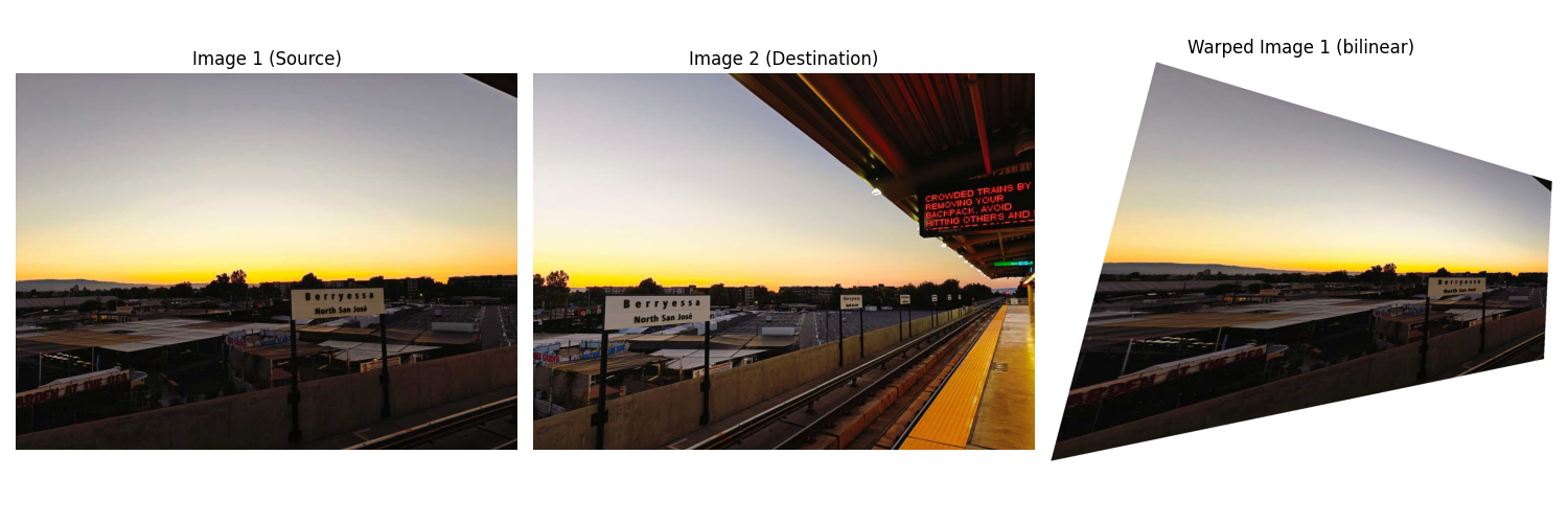
A.3 Warp and Rectify Images

What is Inverse Warping?

Given a source image im and a homography H mapping source pixels to target pixels, the goal is to produce a new image out that shows the source from the target's perspective. The naive forward mapping approach (looping over every pixel in im, applying H, and writing to out) can leave holes because some target pixels may not be hit. Instead, inverse warping loops over every pixel in out, applies the inverse homography H^{-1} to find the corresponding pixel in im, and samples the color there. This guarantees that every pixel in out is filled.

NN vs Bilinear

The NN (nearest neighbour) works like this: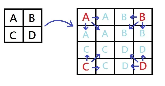

and bilinear interpolation works like this:

A simple view of NN vs bilinear warping of a chessboard pattern is shown below:

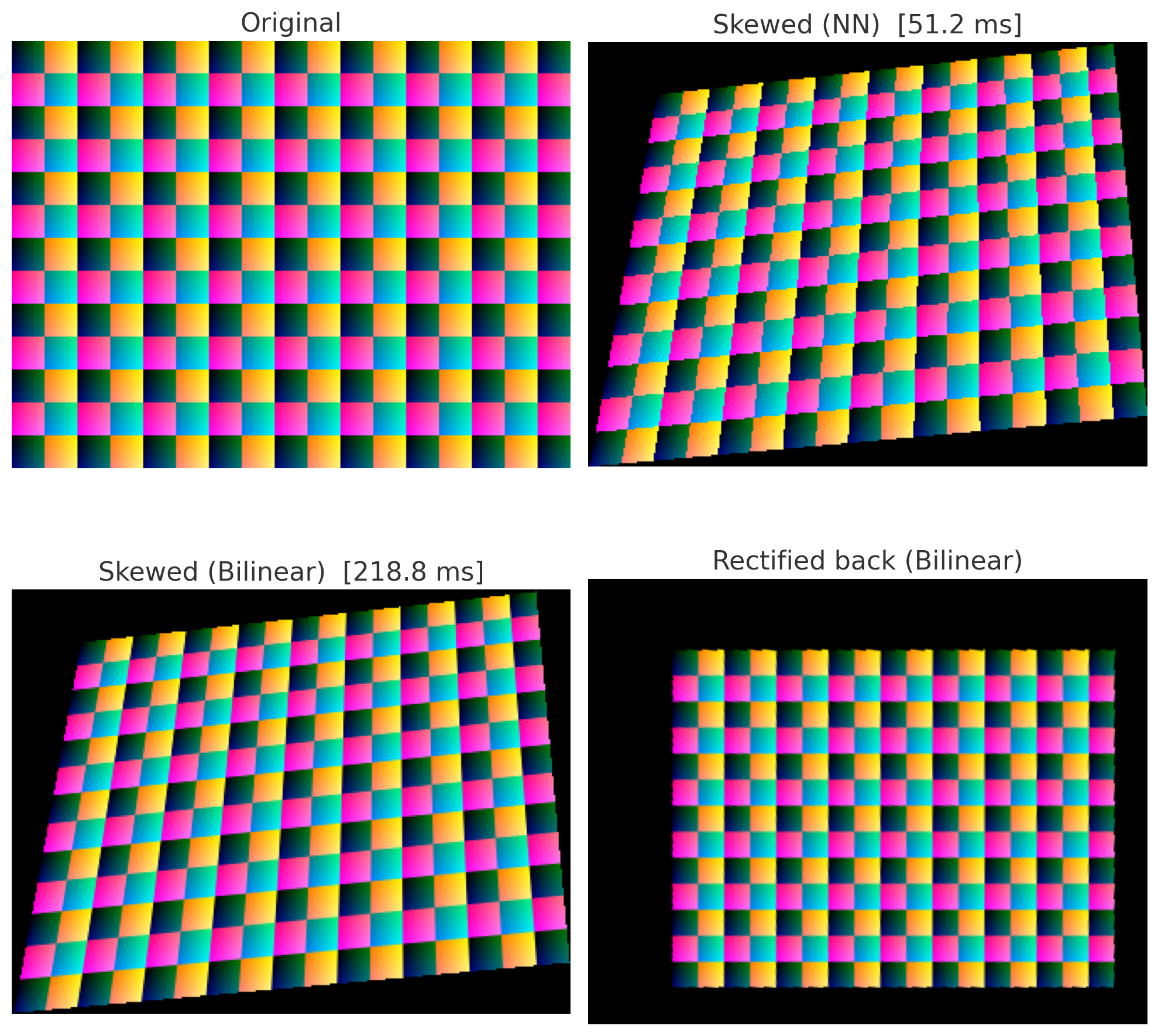
Obviously bilinear is smoother, but NN is faster and avoids introducing new colors (which can be helpful for segmentation). I used bilinear for all final mosaics.

Practical Results

• Bridge:

• Kitchen:

• Station:

A.4 Blend Images into a Mosaic

The mosaicer (blend_utils.build_mosaic) projects every image into a common canvas, warps per-image alpha masks, and blends either by:

• Feathering: simple weighted averaging driven by the warped alpha falloff.
• Laplacian (two-level): blur the alphas, blend low/high bands separately to reduce ghosting.

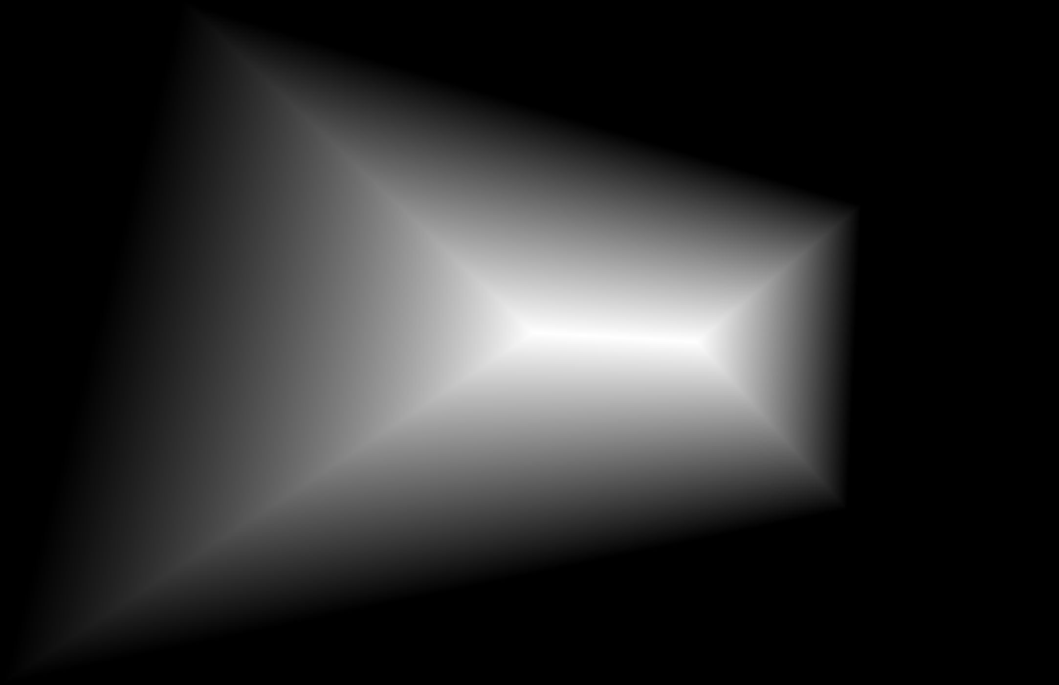
Procedure

1. Unify the coordinate system and canvas size by projecting all image corners and finding the bounding box. That is, multiply H with the four corners, find the final bounding box.

2. Warp each image and its alpha mask into the common canvas using inverse warping.

3. Use a linear falloff alpha mask that is 1 at the center and 0 at the edges, then warp it to the canvas. Shows like this:

   

4. Blend the images using either feathering or Laplacian blending. For Laplacian blending, the low-frequency band is blended with the blurred alpha masks, and the high-frequency band is blended with the sharp alpha masks.

Practical Results

• Bridge (feathering):

• Bridge (Laplacian):

• Kitchen (feathering):

• Kitchen (Laplacian):

• Station (feathering):

• Station (Laplacian):

It's obvious that current manual correspondences are not accurate enough, leading to noticeable artifacts in the blended results. But don't worry, in Part B we will auto detect and match features to get better correspondences.

Further Thoughts

1. I tried to implement spherical warping. The code refers to an open-source implementation here. It works better on Station image:

2. Plan to implement exposure compensation and multi-band blending in next project.

CS180 Lab 3 - Part B

Now no more theory, let's just jump into tasks.

Task 1: Harris Corner Detection

1. Harris Interest Point Detector - single scale: implemented with the given sample code in harris.py.

Results:

Input Image	Detected Corners

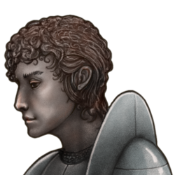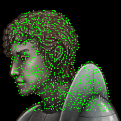
2. Adaptive Non-Maximal Suppression (ANMS)

The key idea of ANMS in the paper is to select corners that are both strong and well-distributed. The algorithm works as follows:

1. Compute the Harris corner response for all pixels in the image. For each corner point, calculate its minimum suppression radius \(r_i\): \[r_i = \min_{j} \{ d_{ij} | h_j > c_{robust} * h_i \}\] where \(d_{ij}\) is the Euclidean distance between corner points \(i\) and \(j\), \(h_i\) and \(h_j\) are their Harris corner responses, and \(c_{robust}\) is a robustness ratio (typically set to 0.9).
2. Sort the corner points by their suppression radii in descending order. The bigger the radius, the more isolated and stronger the corner is.
3. Select the top N corner points with the largest suppression radii.

Results:

Parameters	Detected Corners (ANMS)
N=500, c_robust=0.9
N=300, c_robust=0.9
N=100, c_robust=0.9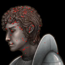
N=500, c_robust=0.7
N=500, c_robust=1.1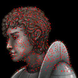

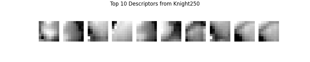
Task 2: Feature Descriptor

The only thing worth mentioning is to bias/gain-normalize the descriptor patch. The equations are as follows:

\[I_{norm} = \frac{I - \mu}{\sigma + \epsilon}\]

where \(\mu\) is the mean intensity of the patch, \(\sigma\) is the standard deviation, and \(\epsilon\) is a small constant (e.g., 1e-10) to prevent division by zero. This normalization ensures that the descriptor is invariant to changes in brightness and contrast, making it more robust for matching features across different images.

So let's just see the results.

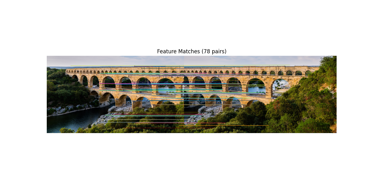
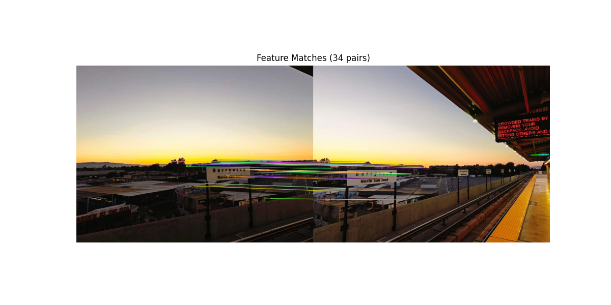
Task 3: Feature Matching

The main idea of the Lowe's ratio test likes this:

1. For each descriptor in the first image \(f_i\), compute the Euclidean distance to all descriptors in the second image \(g_j\).
2. Find the two smallest distances \(d_1\) and \(d_2\).
3. If \(d_1 / d_2 < \text{ratio\_thresh}\), then we consider the match valid.

Why this?

I think the metaphor given by our professor is quite good:

If you are tangling with two boyfriend candidates and cannot decide which one is better, that may indicate that neither of them is really suitable for you. However, if one candidate is clearly better than the other, then you can be more confident in your choice.

Results:

Task 4: Image Stitching with RANSAC

This part is already done in Part A. So let's just see the final results.

manual matches	auto matches with feature matching