线性代数笔记

Preface

The note mainly referenced to MIT 18.06 Linear Algebra, 3blue1brown's Essence of Linear Algebra, and of course, the course of Linear Algebra I in ShanghaiTech University.

Unit 1: Vectors and Matrices

1.1 The Geometry of Linear Equations

What is a matrix?

• 1. a coefficient view(线性方程组的系数):

  \[ \begin{cases} 2x - y = 0\\ -x + 2y = 3 \end{cases} \quad \Rightarrow \quad \begin{bmatrix} 2 & -1\\ -1 & 2 \end{bmatrix} \begin{bmatrix} x\\ y \end{bmatrix} = \begin{bmatrix} 0\\ 3 \end{bmatrix} \]

• 2. a row view(多条线性方程的函数图像): \(\begin{cases} 2x - y = 0\\ -x + 2y = 3 \end{cases}\)

  

• 3. a column view:

  the linear combination of vectors(许多向量的线性组合)

  \[ \begin{bmatrix} 2\\ -1 \end{bmatrix} x + \begin{bmatrix} -1\\ 2 \end{bmatrix} y = \begin{bmatrix} 0\\ 3 \end{bmatrix} \]

• 4. the basis transformation of the space(这一部分将在 Unit3 中的线性变换中给出更详细的解释，但我们应该在一开始就有这样的 intuition)

     将基向量变化为给定矩阵的列向量

1.2 Elimination

Gaussian-Jordan Elimination(高斯-约旦消元法)

所谓消元法，其实可以看作是初中生都会的求解多元一次方程组:

e.g.

\[ \left\{ \begin{array}{rcl} x &+ ~2y + z &= 2 \\ 3x &+ ~8y + z &= 12 \\ & \quad 4y + z &= 2 \end{array} \right. \Rightarrow \left[ \begin{array}{ccc|c} 1 & 2 & 1 & 2 \\ 3 & 8 & 1 & 12 \\ 0 & 4 & 1 & 2 \end{array} \right] \]

这里，我们把方程组等号左边的系数和右边的常数写在一个矩阵中，这个矩阵称为增广矩阵(Augmented Matrix)。

我们应该如何求解这个方程组呢？只看左边的方程组，最直接的思路就是消元法，用第二个方程减去第一个方程，这样就消去了\(z\)，再通过第三个方程得到\(y\)和\(z\)的关系式，最后解出所有的未知数。

高斯消元法的本质就是这样，只不过我们最好按照更加固定的步骤来进行，保证对一切方程组都能按部就班地求解(有了按部就班的方法，剩下的计算就是计算机的活了)。

具体的步骤如下:

• Step 1: 从当前行(第一行)开始，找到第一个非零元素，称为主元素(Pivot)，如果主元素为 0，则交换行，使得主元素不为 0。

  \[ \left[ \begin{array}{ccc|c} \overset{\text{Pivot}}{\fcolorbox{red}{white}{1}} & 2 & 1 & 2 \\ 3 & 8 & 1 & 12 \\ 0 & 4 & 1 & 2 \end{array} \right] \]

• Step 2: 用主元素消去下面的元素，使得下面每一行、同一列(Pivot column)的元素为 0，其他列的元素则加上/减去相应倍数的第一行元素。

  \[ \underset{r_3'=r_3}{\overset{r_2'=r_2-3r_1}{\longrightarrow}} \left[ \begin{array}{ccc|c} 1 & 2 & 1 & 2 \\ 0 & 2 & -2 & 6 \\ 0 & 4 & 1 & 2 \end{array} \right] \]

• Step 3: 换下一行，重复 Step 1 和 Step 2，直到所有的主元素都为 1，且主元素下面的元素都为 0。

  \[ \overset{r_3'=r_3-2r_2}{\longrightarrow} \left[ \begin{array}{ccc|c} {1} & 2 & 1 & 2 \\ 0 & \overset{\text{new Pivot}}{\fcolorbox{red}{white}{2}} & -2 & 6 \\ 0 & 0 & 5 & -10 \end{array} \right] \]

  此时，我们就得到了一个上三角矩阵(Upper Triangular Matrix)，这个矩阵的特点是主对角线以下的元素都为 0 :

  \[ \begin{bmatrix} 1 & 2 & 1\\ \color{red}{0} & 2 & -2\\ \color{red}{0} & \color{red}{0} & 5 \end{bmatrix} \]

  如果我们把这个矩阵的右边的常数项也写在矩阵中，那么这个矩阵就是一个行阶梯形矩阵(Row Echelon Form)：

  

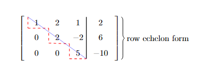
  实际上，到这一步时，我们算是完成了 Gauss-Jordan 消元法的第一部分，也就是"Gaussion Elimination"，即将矩阵变换为上三角矩阵。接下来，我们需要将这个矩阵变换为行最简形矩阵(Row Reduced Echelon Form)。

• Step 4: 回忆最基本的方程组求解办法，现在我们相当于有方程组：

  \[ \begin{cases} x + 2y + z = 2\\ 2y - 2z = 6\\ 5z = -10 \end{cases} \]

  我们应该从最后一行开始，逐步解出所有的未知数，这个过程称为回代(Substitution)。为了方便回代过程，我们可以先把每行归一化：

  \[ \left[ \begin{array}{ccc|c} 1 & 2 & 1 & 2 \\ 0 & 1 & -1 & 3 \\ 0 & 0 & 1 & -2 \end{array} \right] \]

  然后，我们可以模仿一开始的消元过程，从最后一行开始，逐步回代：

  \[ \underset{r_1'=r1-r3}{\overset{r_2' = r_2+r_3}{\longrightarrow}} \left[ \begin{array}{ccc|c} 1 & 2 & 0 & 4 \\ 0 & 1 & 0 & 1 \\ 0 & 0 & 1 & -2 \end{array} \right] \overset{r_1'=r_1-2r_2}{\longrightarrow} \left[ \begin{array}{ccc|c} 1 & 0 & 0 & 2 \\ 0 & 1 & 0 & 1 \\ 0 & 0 & 1 & -2 \end{array} \right] \]

  把这个矩阵变换为行最简形矩阵(Row Reduced Echelon Form)：

  \[ \left[ \begin{array}{ccc|c} \overset{\text{leading} ~1}{\fcolorbox{red}{white}{1}} & 0 & 0 & 2 \\ 0 & \overset{\text{leading} ~1}{\fcolorbox{red}{white}{1}} & 0 & 1 \\ 0 & 0 & \overset{\text{leading} ~1}{\fcolorbox{red}{white}{1}} & -2 \end{array} \right]: \begin{cases} \text{The leading entry in each nonzero row is 1 (called a leading one).} \\ \quad \text{每个非零行的前导元素为 1。} \\ \text{Each leading 1 is the only nonzero entry in its column.} \\ \quad \text{每个前导 1 是其列中唯一的非零元素。} \end{cases} \]

  注意，这个 reduce echelon form 是唯一的，就是我们的方程组的解： $

  \[\begin{cases} x = 2\\ y = 1\\ z = -2 \end{cases}\]

  $

More about Row Ehcelon Form & Reduced Row Echelon Form

• row echelon form 并不一定是 triangular 的，其可以被视为一种弱化或者是推广的 triangular matrix，例如：

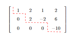
不是 triangular 的 row echelon form

• 一个矩阵消元得到的 row echelon form 并不一定是唯一的，但是 reduced row echelon form 是唯一的。

• 根据 reduced row echelon form 的性质，我们可以把任意的 reduced row echelon form 矩阵写成如下形式：

  \[ \begin{bmatrix} I & X\\ 0 & 0 \end{bmatrix} \]

  其中，\(I\) 是单位矩阵（有且只有主对角线上元素为 1，其余元素为 0），\(X\) 是自由变量的系数矩阵。

1.3 Matrix Multiplication and Inverse

Matrix Multiplication

• 1. 为什么我们需要矩阵乘法？

  在 1.1 中，我们就提到了 coefficient view 和 column view，例如\(\begin{bmatrix}2 & -1\\-1 & 2\end{bmatrix}\begin{bmatrix}x\\y\end{bmatrix}=\begin{bmatrix}0\\3\end{bmatrix}\)，这个式子就是一个矩阵乘法；而我们在 column view 中，也把它理解为两个向量的线性组合，即\(\begin{bmatrix}2\\-1\end{bmatrix}x+\begin{bmatrix}-1\\2\end{bmatrix}y=\begin{bmatrix}0\\3\end{bmatrix}\)，实际上，这两个视角是等价的：矩阵的乘法，都可以视为不同向量的不同线性组合。

• 2. 矩阵乘法的定义：

  对于矩阵\(A\in\mathbb{R}^{m\times \boxed{n}}\)和\(B\in\mathbb{R}^{\boxed{n} \times p}\)，其乘积\(C=AB\in\mathbb{R}^{m\times p}\)的定义为：

  \[ C_{ij}=\sum_{k=1}^nA_{ik}B_{kj} \quad \text{或者说} \quad C_{ij}=\overrightarrow{\text{row}_i(A)}\cdot \overrightarrow{\text{col}_j(B)} \]

  （注：所谓\(A\in\mathbb{R}^{m\times n}\)，表示矩阵\(A\)的行数为\(m\)，列数为\(n\)，所有元素都属于实数域\(\mathbb{R}\)；\(\overrightarrow{\text{row}_i(A)}\)代表将矩阵\(A\)的第\(i\)行视为一个向量）

  很显然，我们发现，矩阵乘法是不满足交换律的，即\(AB\neq BA\)。

• 3. 列视角理解：

  对于矩阵乘法\(AB\)，我们可以把\(A\)视为一组列向量的集合，那么\(AB\)中的每一列都是\(A\)中所有列向量的线性组合，且系数由\(B\)中的对应列决定。

  例如，对于矩阵\(A=\begin{bmatrix}1 & 2\\3 & 4\end{bmatrix}\)和\(B=\begin{bmatrix}5 & 6\\7 & 8\end{bmatrix}\)，我们可以把\(A\)视为两个列向量\(\begin{bmatrix}1\\3\end{bmatrix}\)和\(\begin{bmatrix}2\\4\end{bmatrix}\)，那么\(AB\)中的第一列就是\(A\)中两个列向量的线性组合，而系数则来自\(B\)中对应的第一列元素\(5\)和\(7\)，即\(5\begin{bmatrix}1\\3\end{bmatrix}+7\begin{bmatrix}2\\4\end{bmatrix}=\begin{bmatrix}19\\43\end{bmatrix}\)。同理，\(AB\)中的第二列就是两个列向量以\(B\)中对应的\(6\)和\(8\)为系数的线性组合，即\(6\begin{bmatrix}1\\3\end{bmatrix}+8\begin{bmatrix}2\\4\end{bmatrix}=\begin{bmatrix}22\\50\end{bmatrix}\)。即：

  \[ AB=\begin{bmatrix}1 & 2\\3 & 4\end{bmatrix}\begin{bmatrix}5 & 6\\7 & 8\end{bmatrix}=\begin{bmatrix}19 & 22\\43 & 50\end{bmatrix} \]

• 4. 行视角理解：

  对于矩阵乘法\(AB\)，我们可以把\(B\)视为一组行向量的集合，那么\(AB\)中的每一行都是\(B\)中所有行向量的线性组合，且系数由\(A\)中的对应行决定。

  例如，对于矩阵\(A=\begin{bmatrix}1 & 2\\3 & 4\end{bmatrix}\)和\(B=\begin{bmatrix}5 & 6\\7 & 8\end{bmatrix}\)，我们可以把\(B\)视为两个行向量\(\begin{bmatrix}5 & 6\end{bmatrix}\)和\(\begin{bmatrix}7 & 8\end{bmatrix}\)，那么\(AB\)中的第一行就是\(B\)中两个行向量的线性组合，而系数则来自\(A\)中对应的第一行元素\(1\)和\(2\)，即\(1\begin{bmatrix}5 & 6\end{bmatrix}+2\begin{bmatrix}7 & 8\end{bmatrix}=\begin{bmatrix}19 & 22\end{bmatrix}\)。同理，\(AB\)中的第二行就是两个行向量以\(A\)中对应的\(3\)和\(4\)为系数的线性组合，即\(3\begin{bmatrix}5 & 6\end{bmatrix}+4\begin{bmatrix}7 & 8\end{bmatrix}=\begin{bmatrix}43 & 50\end{bmatrix}\)。即：

  \[ AB=\begin{bmatrix}1 & 2\\3 & 4\end{bmatrix}\begin{bmatrix}5 & 6\\7 & 8\end{bmatrix}=\begin{bmatrix}19 & 22\\43 & 50\end{bmatrix} \]

• 22. 块(block)视角理解：

  如果我们把一个大的矩阵分为几个小的块，那么矩阵乘法就可以看作是块的乘法：

  \[ \begin{bmatrix} A_{11} & A_{12}\\ A_{21} & A_{22} \end{bmatrix} \begin{bmatrix} B_{11} & B_{12}\\ B_{21} & B_{22} \end{bmatrix} = \begin{bmatrix} A_{11}B_{11}+A_{12}B_{21} & A_{11}B_{12}+A_{12}B_{22}\\ A_{21}B_{11}+A_{22}B_{21} & A_{21}B_{12}+A_{22}B_{22} \end{bmatrix} \]

  一种可能的分块：

  \[ \begin{bmatrix} 1 & 2 & 3 & 4\\ 5 & 6 & 7 & 8 \end{bmatrix} \longrightarrow \left[ \begin{array}{cc|cc} 1 & 2 & 3 & 4\\ \hline 5 & 6 & 7 & 8 \end{array} \right] \longrightarrow \begin{bmatrix} A_{11} & A_{12}\\ A_{21} & A_{22} \end{bmatrix} \]

• 6. 高斯消元中的矩阵乘法

  在(III)和(IV)中，我们提到了矩阵乘法的列视角和行视角，为什么我们要这样理解矩阵乘法呢？这是因为在高斯消元法中，我们用一行加上或减去另一行的倍数，实际上就是在做矩阵乘法的行视角理解：

  \[ \left[ \begin{array}{ccc|c} 1 & 2 & 1 & 2 \\ 3 & 8 & 1 & 12 \\ 0 & 4 & 1 & 2 \end{array} \right] \overset{r_2'=r_2-3r_1}{\longrightarrow} \left[ \begin{array}{ccc|c} 1 & 2 & 1 & 2 \\ 0 & 2 & -2 & 6 \\ 0 & 4 & 1 & 2 \end{array} \right] \]

  等价于：

  \[ \underset{E_1}{\begin{bmatrix} 1 & 0 & 0\\ -3 & 1 & 0\\ 0 & 0 & 1 \end{bmatrix}} \underset{A}{\begin{bmatrix} 1 & 2 & 1 & 2 \\ 3 & 8 & 1 & 12 \\ 0 & 4 & 1 & 2 \end{bmatrix}} = \underset{B}{\begin{bmatrix} 1 & 2 & 1 & 2 \\ 0 & 2 & -2 & 6 \\ 0 & 4 & 1 & 2 \end{bmatrix}} \]

  自然地，既然我们可以把“第二行减去三倍的第一行”理解为一个矩阵乘法，那么我们也可以把高斯消元法的所有步骤理解为许多矩阵乘法的组合：

  \[ \underset{\underset{第二步}{E_2}}{\begin{bmatrix} 1 & 0 & 0\\ 0 & 1 & 0\\ 0 & -2 & 1 \end{bmatrix}} \underset{\underset{第一步}{E_1}}{\begin{bmatrix} 1 & 0 & 0\\ -3 & 1 & 0\\ 0 & 0 & 1 \end{bmatrix}} \underset{A}{\begin{bmatrix} 1 & 2 & 1 & 2 \\ 3 & 8 & 1 & 12 \\ 0 & 4 & 1 & 2 \end{bmatrix}} = \underset{U}{\begin{bmatrix} 1 & 2 & 1 & 2 \\ 0 & 2 & -2 & 6 \\ 0 & 0 & 5 & -10 \end{bmatrix}} \]

  这里，\(E_1\)和\(E_2\)分别是高斯消元法的第一步和第二步的矩阵，\(A\)是原始的增广矩阵，\(U\)是上三角矩阵。当然，我们也可以把\(E_1\)和\(E_2\)合并为一个矩阵\(E=E_2E_1\)，那么\(U=EA\)。

  另外，我们很容易能注意到，所有的\(E_i\)都是下三角矩阵(Lower Triangular Matrix)，这很直观，因为我们在消元的过程中，只是用下面的行减去上面的行的倍数，而不会用上面的行减去下面的行的倍数，自然地，\(E\)也是下三角矩阵。

Matrix Inverse

​ 既然我们有了乘法，那么肯定也得有除法吧！（之后我们会从一个更抽象的层面去理解为什么有了乘就得有除）

​ 如何定义矩阵的除法？回忆实数的乘除，\(\frac{a}{b} = ab^{-1} = a \times \mathbf{1} \div b\) ，这看上去好像是废话是不是，但这正是我们对除法最根本的定义：乘以这个数的倒数（Inverse）。而倒数的定义就是，这个数乘以他的倒数等于单位\(\mathbf{1}\)。

​ 那么，在矩阵中，单位一是什么呢？不用说你也应该猜到了，就是我们之前所说的单位矩阵\(\mathbf{I}\)，不过和实数中的1不同的是，\(\mathbf{I}\)并不是一个完全确定的数字，而可以是任意大小(只要符合\(R^{n \times n}\)以及对角线上元素全为\(1\)而其余元素为\(0\)即可)。因此，当我们对任意一个矩阵\(A \in R^{m \times n}\)说\(A^{-1}\)时，其满足： \[ A^{-1}A=\mathbf{I},\quad AA^{-1}=\mathbf{I} \] (注意：\(A^{-1}A \in R^{n \times n}\)而\(AA^{-1} \in R^{m \times m}\)，但出于习惯和方便，我们都简写为\(\mathbf{I}\))